Humans have invented and developed languages to symbolize entities, constructing Matrix that captures the essence of reality. On the other hand, any form of entities can be modelled as number, from natural to complex numbers and from points to objects, which existed long before human civilization. Thereby, the universe itself is inherently number, or in short, all is number.

Mathematics is the study of numbers, so if an entity exists, there exists mathematics to describe it, even if we cannot perceive. This is why we (arguably) refer mathematics as discovery instead of invention and often considered the most fundamental and precise way of describing reality. Mathematics is a vast, diverse and abstract field such that it requires books of worth. Here, a few branches of mathematics are focused on.

Algebra and Calculus

Algebra and calculus are two fundamental highly interconnected branches of mathematics that have been studied and developed for centuries. Algebra deals with equations whereas calculus focuses on functions, but they work together to enable us to solve complex problems and understand the behaviour of functions and systems. Algebra and calculus require a good mathematical foundation to interpret abstract concepts in an intuitive manner.

Algebra

Algebra deals with solving equations and manipulating abstract concepts using mathematical operations and symbols. It involves variables and symbols to perform operations on numbers. It is important for understanding the structure of mathematical systems and solving complex problems.

A System of Linear Equations

A system of linear equations, or linear system, is a collection of one or more linear equations involving the same set of variables. A general system of $m$ linear equations with $n$ unknowns can be written as:

\[\begin{align} a_{11} x_{1} + a_{12} x_{2} + \cdots + a_{1n} x_{n} & = b_{1} \\ a_{21} x_{1} + a_{22} x_{2} + \cdots + a_{2n} x_{n} & = b_{2} \\ & \, \, \vdots \\ a_{m1} x_{1} + a_{m2} x_{2} + \cdots + a_{mn} x_{n} & = b_{m} \end{align}\]

Where $x_{1} , x_{2} , \cdots , x_{n}$ are the unknowns, $a_{11} , a_{12} , \cdots , a_{mn}$ are the coefficients of the system, and $b_{1} , b_{2} , \cdots , b_{m}$ are the constant terms. A linear system can be expressed in different forms:

General form	Vector form	Matrix form
$$ \begin{align} a_{11} x_{1} + \cdots + a_{1n} x_{n} & = b_{1} \\ & \, \, \vdots \\ a_{m1} x_{1} + \cdots + a_{mn} x_{n} & = b_{m} \end{align} $$	$$ \begin{align} x_{1} \begin{bmatrix} a_{11} \\ \vdots \\ a_{m1} \end{bmatrix} + \cdots + x_{n} \begin{bmatrix} a_{1n} \\ \vdots \\ a_{mn} \end{bmatrix} = \begin{bmatrix} b_{1} \\ \vdots \\ b_{m} \end{bmatrix} \end{align} $$	$$ \begin{align} \begin{bmatrix} a_{11} & \cdots & a_{1n} \\ \vdots & \ddots & \vdots \\ a_{m1} & \cdots & a_{mn} \end{bmatrix} \begin{bmatrix} x_{1} \\ \vdots \\ x_{n} \end{bmatrix} = \begin{bmatrix} b_{1} \\ \vdots \\ b_{m} \end{bmatrix} \end{align} $$

Converting the general form to the vector form or the matrix form allows us to apply all the language and theory of vector spaces, or more generally, modules, to be brought in.

An assignment of values to $x_{1} , x_{2} , \cdots , x_{n}$ that simultaneously satisfies all the equations in a linear system is refered to as a solution and the set of all possible solutions is called the solution set. A linear system may behave in any one of three possible ways:

The system has a single unique solution, or the system is always consistent.
The system has infinitely many solutions, or the system is consistent.
The system has no solution, or the system is inconsistent.

If all the constant terms are equal to zero, a system of linear equations is said to be homogeneous.

\[\begin{align} a_{11} x_{1} + a_{12} x_{2} + \cdots + a_{1n} x_{n} & = 0 \\ a_{21} x_{1} + a_{22} x_{2} + \cdots + a_{2n} x_{n} & = 0 \\ & \, \, \vdots \\ a_{m1} x_{1} + a_{m2} x_{2} + \cdots + a_{mn} x_{n} & = 0 \end{align}\]

In homogeneous systems of linear equations, there always exists one trivial solution, that is a zero vector, $x_{1} = \cdots = x_{n} = 0$.

Geometrical interpretation

Each form of a system of linear equations has its geometrical interpretation.

General form: The solution is the intersection between all the hyperplanes drawn from the linear equations.
Vector form: The solution is the linear combination of column vectors, where the unknowns are the weights.
Matrix form: The solution is the initial vector before linear transformation, where the output is the constant.

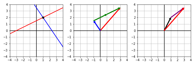
Consider the following three systems of linear equations.

A system of linear equations with a unique solution, $ x = 1 $ and $ y = 2 $.

General form	Vector form	Matrix form
$ \begin{align} - x + 2 y & = 3 \\ 1.5 x + y & = 3.5 \end{align} $	$ \begin{align} x \begin{bmatrix} -1 \\ 1.5 \end{bmatrix} + y \begin{bmatrix} 2 \\ 1 \end{bmatrix} = \begin{bmatrix} 3 \\ 3.5 \end{bmatrix} \end{align} $	$ \begin{align} \begin{bmatrix} -1 & 2 \\ 1.5 & 1 \end{bmatrix} \begin{bmatrix} x \\ y \end{bmatrix} = \begin{bmatrix} 3 \\ 3.5 \end{bmatrix} \end{align} $

Red line: $ - x + 2 y = 3 $ Blue line: $ 1.5 x + y = 3.5 $ Black point: $ ( x , y ) = ( 1 , 2 ) $	Red vector: $ \begin{bmatrix} 3 & 3.5 \end{bmatrix}^{\intercal} $ Blue vector: $ \begin{bmatrix} -1 & 1.5 \end{bmatrix}^{\intercal} $ Green vector: $ \begin{bmatrix} 2 & 1 \end{bmatrix}^{\intercal} $	Red vector: $ \begin{bmatrix} 3 & 3.5 \end{bmatrix}^{\intercal} $ Black vector: $ \begin{bmatrix} x & y \end{bmatrix}^{\intercal} = \begin{bmatrix} 1 & 2 \end{bmatrix}^{\intercal} $ Purple vector: Linear transformation of $ \begin{bmatrix} -1 & 2 \\ 1.5 & 1 \end{bmatrix} $

A system of linear equations with infinitely many solutions.

General form	Vector form	Matrix form
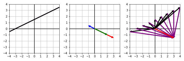
$ \begin{align} - x + 2 y & = 3 \\ 0.5 x - y & = -1.5 \end{align} $	$ \begin{align} x \begin{bmatrix} -1 \\ 0.5 \end{bmatrix} + y \begin{bmatrix} 2 \\ -1 \end{bmatrix} = \begin{bmatrix} 3 \\ -1.5 \end{bmatrix} \end{align} $	$ \begin{align} \begin{bmatrix} -1 & 2 \\ 0.5 & -1 \end{bmatrix} \begin{bmatrix} x \\ y \end{bmatrix} = \begin{bmatrix} 3 \\ -1.5 \end{bmatrix} \end{align} $

Red line: $ - x + 2 y = 3 $ Blue line: $ 0.5 x - y = -1.5 $ Black line: $ - x + 2 y = 3 $ Red and blue line completely overlap, so black line is the solution	Red vector: $ \begin{bmatrix} 3 & -1.5 \end{bmatrix}^{\intercal} $ Blue vector: $ \begin{bmatrix} -1 & 0.5 \end{bmatrix}^{\intercal} $ Green vector: $ \begin{bmatrix} 2 & -1 \end{bmatrix}^{\intercal} $ There are infinitely many linear combinations of red vector	Red vector: $ \begin{bmatrix} 3 & -1.5 \end{bmatrix}^{\intercal} $ Black vector: Infinitely many $ \begin{bmatrix} x & y \end{bmatrix}^{\intercal} $ Purple vector: Linear transformation of $ \begin{bmatrix} -1 & 2 \\ 0.5 & -1 \end{bmatrix} $ per black vector

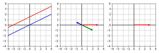
A system of linear equations with no solution.

General form	Vector form	Matrix form
$ \begin{align} - x + 2 y & = 3 \\ 0.5 x - y & = 0 \end{align} $	$ \begin{align} x \begin{bmatrix} -1 \\ 0.5 \end{bmatrix} + y \begin{bmatrix} 2 \\ -1 \end{bmatrix} = \begin{bmatrix} 3 \\ 0 \end{bmatrix} \end{align} $	$ \begin{align} \begin{bmatrix} -1 & 2 \\ 0.5 & -1 \end{bmatrix} \begin{bmatrix} x \\ y \end{bmatrix} = \begin{bmatrix} 3 \\ 0 \end{bmatrix} \end{align} $

Red line: $ - x + 2 y = 3 $ Blue line: $ 0.5 x - y = 0 $ Red and blue line completely separate No black point nor line is present	Red vector: $ \begin{bmatrix} 3 & 0 \end{bmatrix}^{\intercal} $ Blue vector: $ \begin{bmatrix} -1 & 0.5 \end{bmatrix}^{\intercal} $ Green vector: $ \begin{bmatrix} 2 & -1 \end{bmatrix}^{\intercal} $ There is no posssible linear combination of red vector	Red vector: $ \begin{bmatrix} 3 & 0 \end{bmatrix}^{\intercal} $ No black nor purple vector is present

Therefore, in summary:

General form: The solution is the intersection between two lines drawn from two linear equations.
Vector form: The solution is the linear combination of two column vectors, where the unknowns are the number of column vectors required to form the constant terms.
Matrix form: The solution is the black vector before linear transformation, where the red vector is the output and the purple vector is how the black vector transforms into the red vector.

These geometrical interpretations can easily be extended to multi-dimensional space.

Elementary Row Operation

An elementary row operation is a basic operation that can be performed on the rows of a matrix, which results in a new matrix that is equivalent to the original matrix. An operation that converts a matrix into an upper triangular form, in which the coefficients below the main diagonal are zero, is called Gaussian elimination. Consider a system of linear equations with a unique solution, $x = 1$ and $y = 2$.

\[\begin{align} \begin{bmatrix} -1 & 2 \\ 1.5 & 1 \end{bmatrix} \begin{bmatrix} x \\ y \end{bmatrix} = \begin{bmatrix} 3 \\ 3.5 \end{bmatrix} \quad \rightarrow \quad \begin{bmatrix} 1 & -2 \\ 0 & 1 \end{bmatrix} \begin{bmatrix} x \\ y \end{bmatrix} = \begin{bmatrix} -3 \\ 2 \end{bmatrix} \end{align}\]

Gauss-Jordan elimination is an operation that further transforms a matrix into the identity matrix.

\[\begin{align} \begin{bmatrix} 1 & -2 \\ 0 & 1 \end{bmatrix} \begin{bmatrix} x \\ y \end{bmatrix} = \begin{bmatrix} -3 \\ 2 \end{bmatrix} \quad \rightarrow \quad \begin{bmatrix} 1 & 0 \\ 0 & 1 \end{bmatrix} \begin{bmatrix} x \\ y \end{bmatrix} = \begin{bmatrix} 1 \\ 2 \end{bmatrix} = \begin{bmatrix} x \\ y \end{bmatrix} \end{align}\]

After Gauss-Jordan elimination, the geometric representations are:

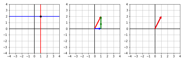
A system of linear equations with a unique solution, $ x = 1 $ and $ y = 2 $, before and after Gauss-Jordan elimination.

General form	Vector form	Matrix form
$ \begin{align} - x + 2 y & = 3 \\ 1.5 x + y & = 3.5 \end{align} $	$ \begin{align} x \begin{bmatrix} -1 \\ 1.5 \end{bmatrix} + y \begin{bmatrix} 2 \\ 1 \end{bmatrix} = \begin{bmatrix} 3 \\ 3.5 \end{bmatrix} \end{align} $	$ \begin{align} \begin{bmatrix} -1 & 2 \\ 1.5 & 1 \end{bmatrix} \begin{bmatrix} x \\ y \end{bmatrix} = \begin{bmatrix} 3 \\ 3.5 \end{bmatrix} \end{align} $

$ \begin{align} x & = 1 \\ y & = 2 \end{align} $	$ \begin{align} x \begin{bmatrix} 1 \\ 0 \end{bmatrix} + y \begin{bmatrix} 0 \\ 1 \end{bmatrix} = \begin{bmatrix} 1 \\ 2 \end{bmatrix} \end{align} $	$ \begin{align} \begin{bmatrix} 1 & 0 \\ 0 & 1 \end{bmatrix} \begin{bmatrix} x \\ y \end{bmatrix} = \begin{bmatrix} 1 \\ 2 \end{bmatrix} \end{align} $

Therefore, manipulating concepts on the space can be seen as equivalent form of handling a linear system in the world of equations. Vector space is particularly useful in solving linear systems since it provides different views from geometrics.

Note that an upper triangular matrix and the identity matrix can only appear if the matrix is a square matrix and the linear system is always consistent. In the case of a rectangular matrix, a consistent linear system or an inconsistent linear system, the matrix is transformed into reduced row echelon form.

Consider a linear system with infinitely many solutions.

\[\begin{equation} \begin{bmatrix} 3 & -2 & 1 \\ 0 & 2 & 2 \\ -1 & 1 & 0 \\ \end{bmatrix} \begin{bmatrix} x \\ y \\ z \\ \end{bmatrix} = \begin{bmatrix} 19 \\ 8 \\ -5 \\ \end{bmatrix} \quad \rightarrow \quad \begin{bmatrix} 1 & 0 & 1 \\ 0 & 1 & 1 \\ 0 & 0 & 0 \\ \end{bmatrix} \begin{bmatrix} x \\ y \\ z \\ \end{bmatrix} = \begin{bmatrix} 9 \\ 4 \\ 0 \\ \end{bmatrix} \end{equation}\]

This can be re-expressed as:

\[\begin{equation} \begin{bmatrix} 1 & 0 & 1 \\ 0 & 1 & 1 \\ \end{bmatrix} \begin{bmatrix} x \\ y \\ z \\ \end{bmatrix} = \begin{bmatrix} 9 \\ 4 \\ \end{bmatrix} \quad \rightarrow \quad \begin{aligned} y & = 5 + x \\ z & = 4 - x \\ \end{aligned} \end{equation}\]

Similarly, consider a linear system with no solution.

\[\begin{equation} \begin{bmatrix} 3 & -2 & 1 \\ 0 & 2 & 2 \\ -1 & 1 & 0 \\ \end{bmatrix} \begin{bmatrix} x \\ y \\ z \\ \end{bmatrix} = \begin{bmatrix} 19 \\ 8 \\ -10 \\ \end{bmatrix} \quad \rightarrow \quad \begin{bmatrix} 1 & 0 & 1 \\ 0 & 1 & 1 \\ 0 & 0 & 0 \\ \end{bmatrix} \begin{bmatrix} x \\ y \\ z \\ \end{bmatrix} = \begin{bmatrix} 9 \\ 4 \\ -5 \\ \end{bmatrix} \end{equation}\]

Since $0 x + 0 y + 0 z \neq -5$, the linear system is inconsistent.

Calculus

Calculus deals with rates of change and slopes of curves. It involves limits, derivatives, and integrals to understand how things change over time or space. It is important for understanding complex systems and modeling real-world phenomena.

Function

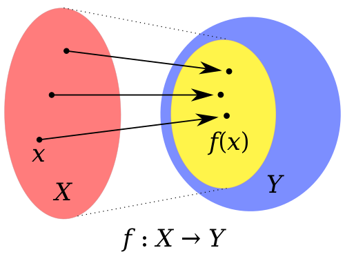
A function is a process or a relation that associates the domain of the function, or the set of inputs, to the codomain of the function, or the set of outputs. It can be visualized as:

$\mathcal{X}$ is the domain of a function and its element is $x \in \mathcal{X}$.
$\mathcal{Y}$ is the codomain of a function.
$f$ is a function that maps from $\mathcal{X}$ to $\mathcal{Y}$, commonly denoted as $f : \mathcal{X} \rightarrow \mathcal{Y}$, or $y = f ( x )$.
$x$ is referred to as the input, or the argument of $f$.
$f ( x )$ is referred to as the output, or the image of $f$.
$f ( x )$ and $\mathcal{Y}$ may not coincide, $f ( x ) \subseteq \mathcal{Y}$.

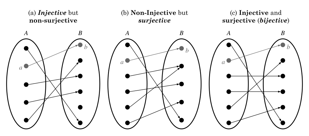
There exist a few classes of $f$.

Injection: Each element of the codomain is mapped to at most one element of the domain, or one-to-one. Formally, $\forall x , x' \in \mathcal{X} , f(x) = f(x') \implies x = x'$.
Surjection: Each element of the codomain is mapped to at least one element of the domain, or onto. Formally, $\forall y \in \mathcal{Y} , \exists x \in \mathcal{X}$ such that $y = f(x)$.
Bijection: Each element of the codomain is mapped to exactly one element of the domain, or one-to-one correspondence or invertible. Formally, $\forall y \in \mathcal{Y} , \exists !x \in \mathcal{X}$ such that $y = f(x)$.

There are two additional classes of $f$.

A function can be neither injective, surjective nor bijective. If so, each element of the codomain is mapped to any number of elements of the domain. Formally, $\forall x \in \mathcal{X} , \exists !y \in \mathcal{Y}$ such that $y = f(x)$.
A function cannot have a condition that two or more elements of the codomain is mapped to any number of elements of the domain. This is not considered as a function.

Types of $f$ vary by how $x$ is mapped to $f ( x )$.

Linear function: $f ( x ) = a x + b$
Polynomial function: $f ( x ) = \sum_{i=0}^{n} a_{i} x^{i}$
Power function: $f ( x ) = a x^{b}$
Exponential function: $f ( x ) = a e^{x}$
Logarithmic function: $f ( x ) = a \ln ( x ) + b$

Continuity

A function $f$ is continuous at a point $a \in \mathcal{X}$ if its value approaches $f ( a )$ when its argument approaches $a$. If $f$ is continuous at every point, or if it maps a continuous domain to a continuous codomain, it is referred to as continuous function.

More formally, a function $f : \mathcal{X} \rightarrow \mathbb{R}$ is continuous at $a \in \mathcal{X}$ if:

\[\begin{equation} \lim_{x \rightarrow c} f ( x ) = f ( c ) \end{equation}\]

A continuity indicates no abrupt change, or no jump, in its value.
A discontinuity indicates an abrupt change, or a jump, in its value.
A point or a region can be continuous in discontinuous function.

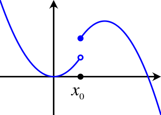
A discontinuous function classes from Wikimedia Commons
- A function at any $x$ greater than or equal to $x_{0}$ is continuous.

The continuity of $f$ can be generalized to a metric space. A metric space is a space of a metric function, which measures the distance between any two elements in $\mathcal{X}$, $d_{\mathcal{X}} : \mathcal{X} \times \mathcal{X} \rightarrow \mathbb{R}$.

Given two metric spaces $\left( \mathcal{X} , d_{\mathcal{X}} \right)$ and $\left( \mathcal{Y} , d_{\mathcal{Y}} \right)$, and a function $f : \mathcal{X} \rightarrow \mathcal{Y}$ is continuous at the point $x_{0} \in \mathcal{X}$ with respect to the given metrics if for every $\epsilon > 0$, there exists $\delta > 0$, such that all $x \in \mathcal{X}$ satisfying $d_{\mathcal{X}} (x , x_{0}) < \delta$ implies $d_{\mathcal{Y}} (f(x) , f(x_{0})) < \epsilon$.

The strength of the continuity in metric space exists and is determined by constraining $\delta$ with $x_{0}$ and $\epsilon$.

Uniformly continuous if $d_{\mathcal{X}} (x , x_{0}) < \delta$ and $d_{\mathcal{Y}} (f(x) , f(x_{0})) < \epsilon$.
Lipschitz continuous if $d_{\mathcal{Y}} (f(x) , f(x_{0})) \leq K \cdot d_{\mathcal{X}} (x , x_{0})$, where $K \in \mathbb{R}$. Any Lipschitz continuous function is uniformly continuous.
Holder continuous if $d_{\mathcal{Y}} (f(x) , f(x_{0})) \leq K \cdot ( d_{\mathcal{X}} (x , x_{0}) )^{a}$, where $K \in \mathbb{R}$ and $a \in \mathbb{R}$. Any Holder continuous function is uniformly continuous and if $a = 1$, it is Lipschitz continuous.

Differentiability

A function $f$ is differentiable at a point $a \in \mathcal{X}$ if derivative exists at $a$. If a function $f$ is differentiable at every point, it is referred to as differentiable function.

A tangent to the curve from Wikimedia Commons

More formally, a function $f : \mathcal{X} \rightarrow \mathbb{R}$ is differentiable at $a \in \mathcal{X}$ if:

\[\begin{equation} f' (a) = \lim_{h \rightarrow 0} \frac{ f (a + h) - f (a) }{ h } \end{equation}\]

A point or a region can be differentiable in non-differentiable function.
A function $f$ is said to be continuously differentiable if its derivative is also a continuous function.
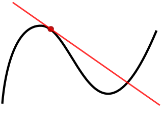
If a function $f$ is differentiable at $a$, $f$ is continuous at $a$, but not vice versa. For instance, $f$ with a bend, cusp, or vertical tangent may be continuous, but fails to be differentiable at the location of the anomaly.
From a tangent line point-of-view, a function $f$ is differentiable at a point $a$ if it has a non-vertical tangent line at the point $(a, f(a))$. Furthermore, $f$ is differentiable function if it has a non-vertical tangent line at every point.

There is a differentiability class, $C^{k}$, that measures the highest order of derivative that exists and is continuous over $\mathcal{X}$. If $f' (x), f'' (x), \cdots, f^{(k)} (x)$ exist and are continuous, a function $f$ is said to be of differentiability class, $C^{k}$.

If a function $f$ is $k$-differentiable, $f' (x), f'' (x), \cdots, f^{(k-1)} (x)$, $f$ is at least of the class $C^{k-1}$.
If a function $f$ is infinitely differentiable, $f' (x), f'' (x), \cdots, f^{(\infty)} (x)$, $f$ is of class $C^{\infty}$.
If a function $f$ is of class $C^{\infty}$, $f$ is said to be infinitely differentiable, or smooth.

Intuitively:

The class $C^{0}$ consists of all continuous functions.
The class $C^{1}$ consists of all continuously differentiable functions that its derivative is of class $C^{0}$.
The class $C^{k}$ consists of all continuously differentiable functions that its derivative is of class $C^{k-1}$.

Probability and Statistics

Probability and statistics are two interconnected fields of study that play a critical role in making sense of data and uncertainty in various disciplines. To simply put, probability is about the idea of formalizing uncertainty while statistics is about the idea of analyzing the data, so often, statistics is considered as an applied probability to the data. Probability and statistics require a slightly different way to look at things since probabilistic arguments are often built up with apparently paradoxical or counterintuitive results.

Probability

Probability deals with random events and the likelihood of their occurrence. It involves the chance of different outcomes based on the possible outcomes as well as the conditions or assumptions of the situation. It is important for understanding risk, uncertainty, and decision-making under uncertainty.

Combinatorics

Combinatorics is a branch of mathematics that focuses on the study of finite or countable discrete structures. It deals with the arrangement, combination, and selection of objects, elements, or sets. Combinatorics is not usually used in probability theory, but it is the fundamentals for understanding the likelihood.

There are two simplest ways to count the number of possible arrangements given a set with $n$ size based on repetition, or replacement or duplicates.

A factorial is used to compute the arrangements without repetition, $n! = 1$ if $n = 0$, otherwise, $n! = \Pi_{i = 1}^{n} i = n \times ( n - 1 ) \times \cdots \times 1$.
A power is used to compute the arrangements with repetition, $n^{n} = n \times n \times \cdots \times n$.

For instance, if a set consists of $S = \{ 1 , 2 , 3 , 4 \}$, the possible arrangements without repetition is $4! = 24$ and with repetition is $4^{4} = 256$.

The application of a factorial and power extends to more complex problems. Consider that we are selecting $4$ elements from a set, $S = \{ 1 , 2 , 3 , 4 , 5 , 6 , 7 \}$. There are four types of common problems in combinatorics.

The arrangements of $r$ number of elements from a set with $n$ size in order without repetition.
- If we were to arrange $7$ elements in order and consider only the first $r = 4$ elements, the following arrangements are essentially the same:
  \[\begin{equation} ( 1 , 2 , 3 , 4 \vert 5 , 6 , 7 ) \equiv ( 1 , 2 , 3 , 4 \vert 7 , 6 , 5 ) \end{equation}\]
- Then, this means that we ought to remove all the arrangements of the last three elements given the first four elements, $\frac{ \text{Total N of arrangements} }{ \text{N of removal arrangements} } = \frac{ 7 \times 6 \times 5 \times 4 \times 3 \times 2 \times 1 }{ 3 \times 2 \times 1 }$. This can be generalized as:
  \[\begin{align} \frac{ n! }{ ( n - r )! } & = \frac{ n \times ( n - 1 ) \times \cdots \times ( n - r + 1 ) \times ( n - r ) \times \cdots \times 1 }{ ( n - r ) \times \cdots \times 1 } \\ & = P_{r}^{n} = P ( n , r ) \end{align}\]
- Where $P_{r}^{n}$ is referred to as a permutation. Due to this, the problem is often referred to as a permutation without repetition.
The arrangements of $r$ number of elements from a set with $n$ size in order with repetition.
- $n^{n}$ can be seen as filling up $n$ number of elements in $n$ number of slots with repetition. Since the goal is to fill $4$ slots with repetition, it is as simple as $n^{r} = 7^{4}$.
- Although it does not use the permutation directly, the problem is often referred to as a permutation with repetition.
The arrangements of $r$ number of elements from a set with $n$ size not in order without repetition.
- If we were to arrange $7$ elements in order and consider only the first $r = 4$ elements, the following arrangements are essentially the same:
  \[\begin{equation} ( 1 , 2 , 3 , 4 \vert 5 , 6 , 7 ) \equiv ( 1 , 2 , 3 , 4 \vert 7 , 6 , 5 ) \equiv ( 4 , 3 , 2 , 1 \vert 5 , 6 , 7 ) \equiv ( 4 , 3 , 2 , 1 \vert 7 , 6 , 5 ) \end{equation}\]
- Then, this means that we ought to remove all the arrangements of the last three elements given the first four elements as well as the equivalent arrangements of the first four elements, $\frac{ \text{Total N of arrangements} }{ \text{N of removal arrangements} } = \frac{ 7 \times 6 \times 5 \times 4 \times 3 \times 2 \times 1 }{ ( 4 \times 3 \times 2 \times 1 ) \times ( 3 \times 2 \times 1 ) }$. This can be generalized as:
  \[\begin{align} \frac{ n! }{ r! ( n - r )! } & = \frac{ n \times ( n - 1 ) \times ( n - 2 ) \times \cdots \times ( n - r + 1 ) \times ( n - r ) \times \cdots \times 1 }{ ( r \times ( r - 1 ) \times \cdots \times 1 ) \times ( ( n - r ) \times \cdots \times 1 ) } \\ & = \frac{ P_{r}^{n} }{ r! } = C_{r}^{n} = C ( n , r ) = \begin{pmatrix} n \\ r \end{pmatrix} \end{align}\]
- Where $C_{r}^{n}$ is referred to as a combination. Due to this, the problem is often referred to as a combination without repetition.
  - Note that the following expressions of $C_{r}^{n}$ are equivalent:
    \[\begin{align} \begin{pmatrix} n \\ r \end{pmatrix} & = \frac{ n! }{ r! ( n - r )! } = \frac{ n! }{ ( n - n + r )! ( n - r )! } \\ & = \frac{ n! }{ ( n - r )! ( n - ( n - r ) )! } = \begin{pmatrix} n \\ n - r \end{pmatrix} \end{align}\]
- One application of $C_{r}^{n}$ is the arrangements of entire elements from a multiset. For instance, if a multiset consists of $S' = \{ A , A , B , B , B \}$, the possible arrangements of entire elements can be formalized as a combination with $n = 5$ and $r = 2$.
  \[\begin{equation} \begin{pmatrix} 5 \\ 2 \end{pmatrix} = \frac{ 5! }{ 2! ( 5 - 2 )! } = \frac{ 5! }{ ( 5 - 3 )! 3! } = \begin{pmatrix} 5 \\ 3 \end{pmatrix} \end{equation}\]
  - This can be generalized with the multinomial coefficient:
  \[\begin{equation} \begin{pmatrix} n \\ r_{1} , r_{2} , \cdots , r_{m} \end{pmatrix} = \frac{ n! }{ r_{1}! r_{2}! \cdots r_{m}! } \end{equation}\]
  - Where $n$ is the size of a multiset and $r_{i}$ is the type of elements.
The arrangements of $r$ number of elements from a set with $n$ size not in order with repetition.
- The intuition behind this is slightly different from other problems. Here, we define a set as:
  \[\begin{equation} S' = \{ \text{O} , \text{O} , \text{O} , \text{O} , \vert , \vert , \vert , \vert , \vert , \vert \} \end{equation}\]
- Where $\vert$ is a separator that distributes O to into $7$ subsets, which is of the original set, $S = \{ 1 , 2 , 3 , 4 , 5 , 6 , 7 \}$. For instance:
  \[\begin{equation} ( \text{O} , \text{O} , \text{O} , \text{O} , \vert , \vert , \vert , \vert , \vert , \vert ) \quad \rightarrow \quad ( 1 , 1 , 1 , 1 , \vert , \vert , \vert , \vert , \vert , \vert ) \quad \rightarrow \quad ( 1 , 1 , 1 , 1 ) \\ ( \text{O} , \text{O} , \vert , \text{O} , \vert , \text{O} , \vert , \vert , \vert , \vert ) \quad \rightarrow \quad ( 1 , 1 , \vert , 2 , \vert , 3 , \vert , \vert , \vert , \vert ) \quad \rightarrow \quad ( 1 , 1 , 2 , 3 ) \\ ( \vert , \text{O} , \vert , \text{O} , \text{O} , \vert , \vert , \vert , \vert , \text{O} ) \quad \rightarrow \quad ( \vert , 2 , \vert , 3 , 3 , \vert , \vert , \vert , \vert , 7 ) \quad \rightarrow \quad ( 2 , 3 , 3 , 7 ) \end{equation}\]
- This enables us to simplify the problem into arrangements of entire elements from a multiset, where two types are either $\text{O}$ or $\vert$. Therefore, this results in $\begin{pmatrix} 10 \\ 4 \end{pmatrix} = \begin{pmatrix} 7 + 4 - 1 \\ 4 \end{pmatrix} = \frac{ 10! }{ 4! ( 10 - 4 )! }$. This can be generalized as:
  \[\begin{align} \frac{ ( n + r - 1 )! }{ r! ( ( n + r - 1 ) - r )! } & = \frac{ ( n + r - 1 )! }{ r! ( n - 1 )! } = \begin{pmatrix} n + r - 1 \\ r \end{pmatrix} = \begin{pmatrix} n + r - 1 \\ n - 1 \end{pmatrix} \\ & = \frac{ P_{r}^{n + r - 1} }{ r! } = C_{r}^{n + r - 1} = C ( n + r - 1 , r ) \end{align}\]
- The problem is often referred to as a combination with repetition.

Probability Theory

A probability deals with the quantification of the likelihood of an event occurring, which an event refers to a set of possible outcomes. A probability space, or probability triple, $( \Omega , \mathcal{F} , P )$, is a mathematical framework that describes a set of possible outcomes or events, along with their associated probabilities.

$\Omega$ is a sample space.
$\mathcal{F}$ is an event space, which is a subsets of $\Omega$, such that $\Omega \in \mathcal{F}$ and $\vert \mathcal{F} \vert = 2^{ \vert \Omega \vert } = \sum_{r = 0}^{\vert \Omega \vert} \begin{pmatrix} n \\ r \end{pmatrix}$.
$P$ is a probability function, mapping from $\mathcal{F}$ to a probability. It is noted $P : \mathcal{F} \rightarrow [ 0 , 1 ]$, where $P ( \Omega ) = 1$.

Where $\Omega$ can be considered as a set in combinatorics and $\mathcal{F}$ as a collection of arrangements across different element number under a combination without repetition. If $\Omega = \{ 1 , 2 \}$, then $\mathcal{F} = \{ ( ) , ( 1 ) , ( 2 ) , ( 1 , 2 ) \}$.

The probability axioms, or Kolmogorov axioms, are the three fundamental axioms in probability theory. Let $E$ be an event, $\forall E \in F$:

The probability of an event is a non-negative real number: $P ( E ) \in \mathbb{R} , P ( E ) \geq 0$.
The probability that at least one of the elementary events in the entire sample space will occur is 1: $P ( \Omega ) = 1$.
Any countable sequence of mutually exclusive events, $E_{i}$, satisfies: $P \left( \bigcup_{i = 1}^{\infty} E_{i} \right) = \sum_{i = 1}^{\infty} P ( E_{i} )$.

Any probability must satisfy $P ( E ) \in [ 0 , 1 ]$, where $X$ is a random event, where $P ( E ) = 0$ represents impossibility and $P ( E ) = 1$ indicates certainty.

There are few types of probabilities. Let the sample space be $\Omega = \{ A , B \}$.

Event	Probability
$ A $	$ \begin{align} P ( A ) \in [ 0 , 1 ] \end{align} $
not $ A $	$ \begin{align} P ( A' ) = 1 - P ( A ) \end{align} $
$ A $ or $ B $	$ \begin{align} P ( A \cup B ) & = P ( A ) + P ( B ) - P ( A \cap B ) \\ P ( A \cup B ) & = P ( A ) + P ( B ) \quad \text{if $$ A $$ and $$ B $$ are mutually exclusive} \end{align} $
$ A $ and $ B $	$ \begin{align} P ( A \cap B ) & = P ( A , B ) = P ( A \vert B ) P ( B ) = P ( B \vert A ) P ( A ) \\ P ( A \cap B ) & = P ( A , B ) = P ( A ) P ( B ) \quad \text{if $$ A $$ and $$ B $$ are independent} \end{align} $
$ A $ given $ B $	$ \begin{align} P ( A \vert B ) = \frac{ P ( A \cap B ) }{ P ( B ) } = \frac{ P ( B \vert A ) P ( A ) }{ P ( B ) } \quad \text{if $$ A $$ and $$ B $$ are dependent} \end{align} $

Two important conditions are:

Mutually exclusive events: Events can only occur separately, not simultaneously.
Independent events: Occuring one event do not interfere the probability of other events occuring.

One important concept is the Bayes theorem.

\[\begin{equation} P ( A \vert B ) = \frac{ P ( A \cap B ) }{ P ( B ) } = \frac{ P ( B \vert A ) P ( A ) }{ P ( B ) } \end{equation}\]

$P ( A )$ is referred to as a prior proability.
$P ( B )$ is referred to as an marginal proability, or evidence.
$P ( A \cap B )$ is referred to as a joint probability.
$P ( B \vert A )$ is referred to as a conditional probability, or likelihood.
$P ( A \vert B )$ is referred to as a posterior probability, which is also a conditional probability.

The Bayes theorem can only be applied if $A$ and $B$ are dependent since if they are independent, there is no conditional probability between two random variables, $P ( A \vert B ) = P ( A )$ and $P ( B \vert A ) = P ( B )$.

\[\begin{equation} P ( A \vert B ) = \frac{ P ( B \vert A ) P ( A ) }{ P ( B ) } \quad \rightarrow \quad P ( A ) = \frac{ P ( B ) P ( A ) }{ P ( B ) } = P ( A ) \end{equation}\]

Bayes theorem is also heavily used in statistics since it provides a way to update the probability of an event or hypothesis based on new evidence or data.

Intuition behind Probability Theory

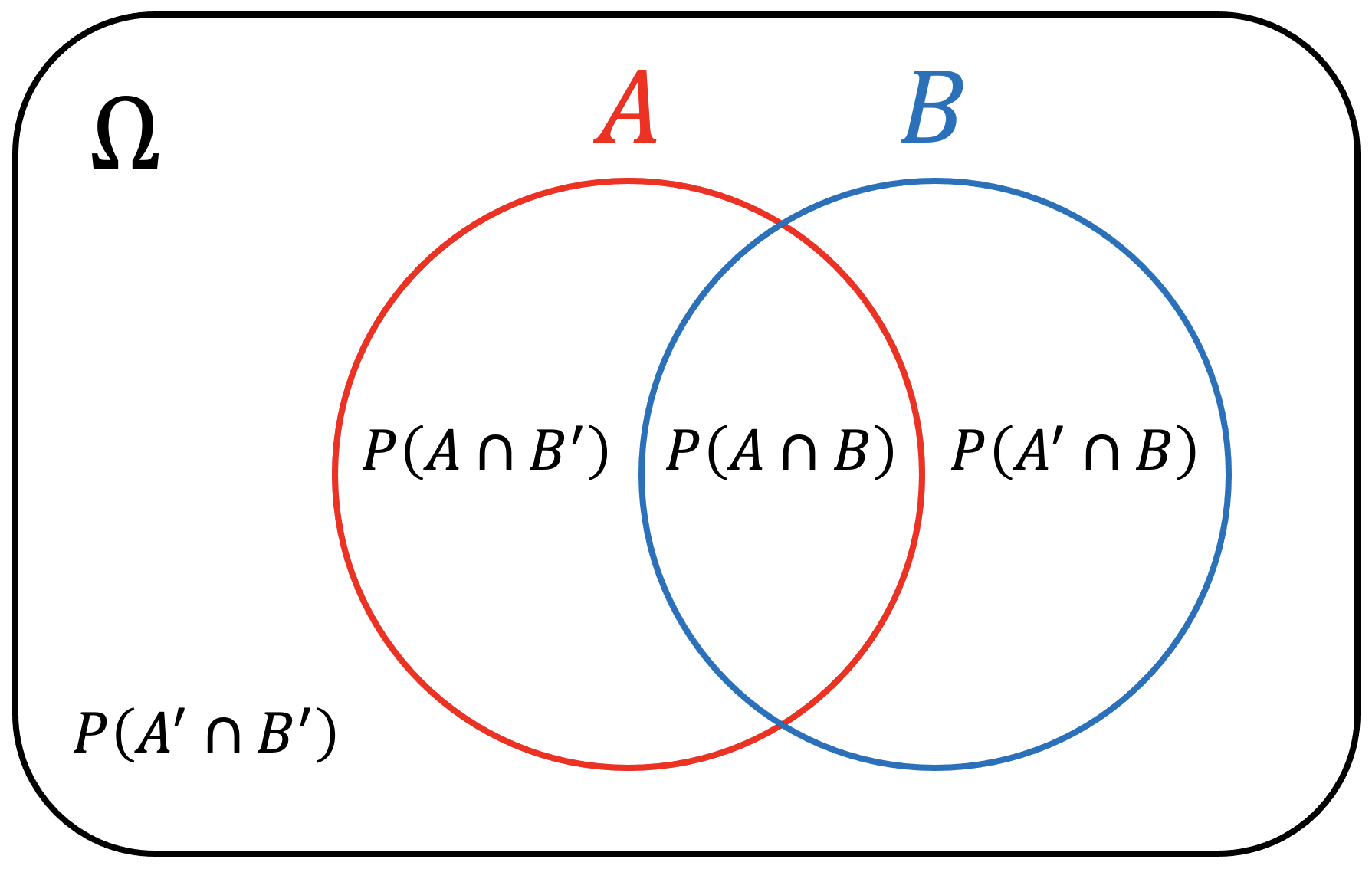
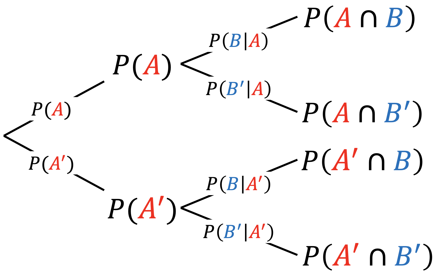
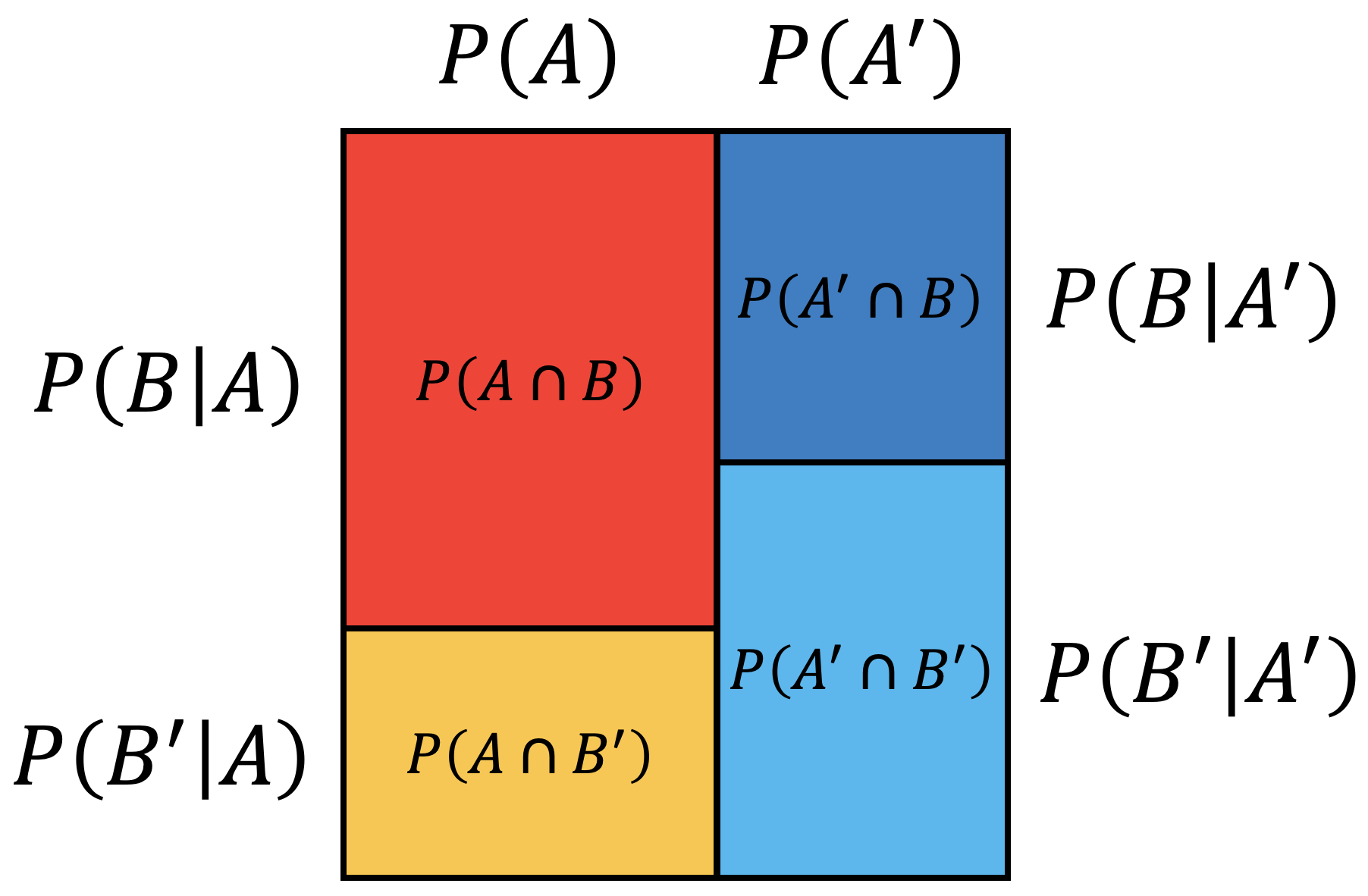
There are three ways to visualize probability using different diagrams.

Venn diagram	Tree diagram	Square diagram

A Venn diagram is intuitive to visualize mutually exclusive events while a tree diagram and square diagram are useful for independent events.

In a Venn diagram, if $A$ and $B$ do not overlap, they are mutually exclusive events.
In a tree and square diagram, if $P ( B \vert A ) = P ( B \vert A' )$, $A$ and $B$ are independent events.

Another intuition behind probability theory is that a probability is just a measure of the target outcomes out of all the possible outcomes.

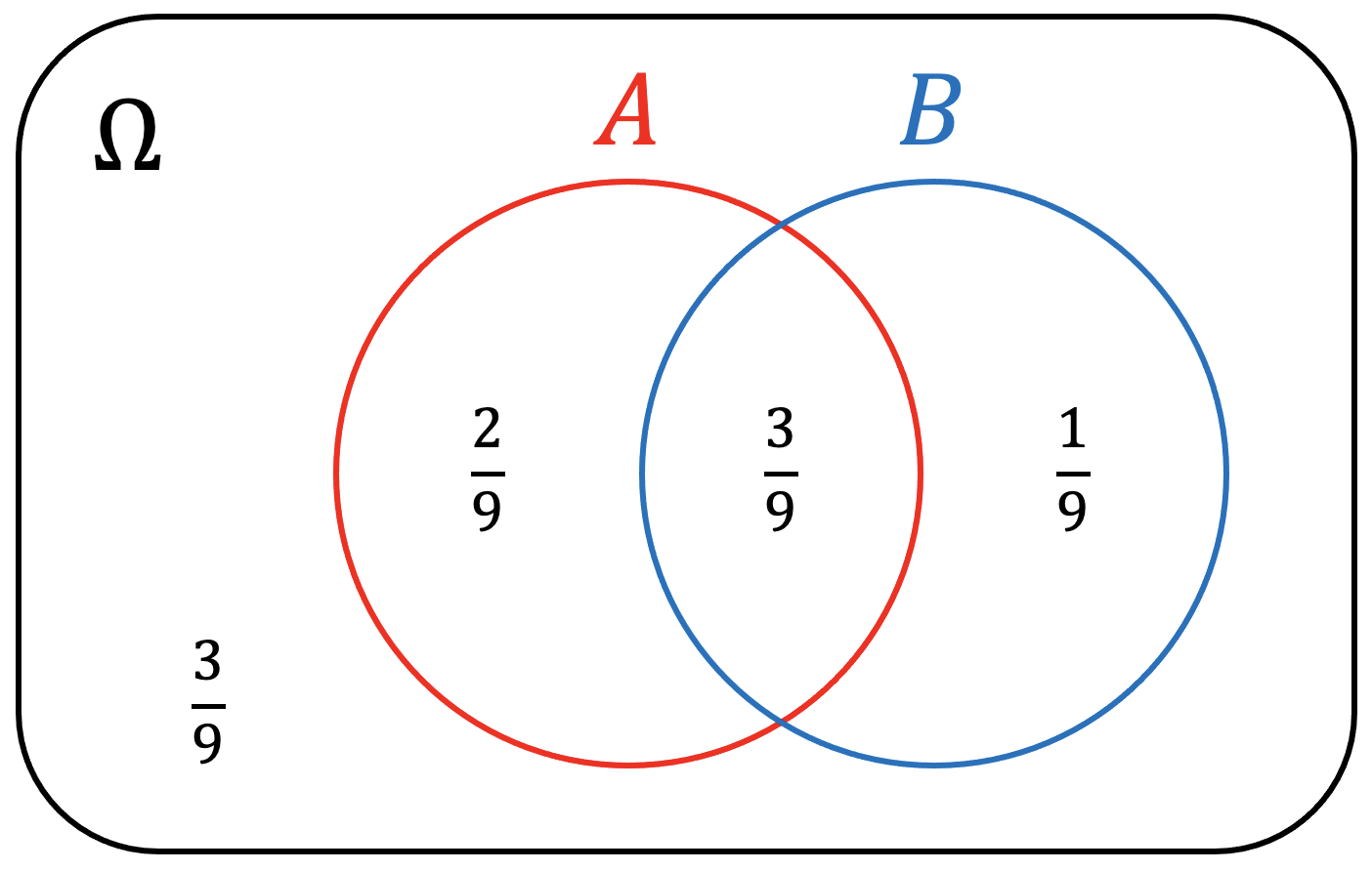
Consider a problem with a set of $\Omega = \{ 1, 2, 3, 4, 5, 6, 7, 8, 9 \}$, where there are two types of classes, odd numbers, $A$, and prime numbers, $B$. A Venn diagram of this is:

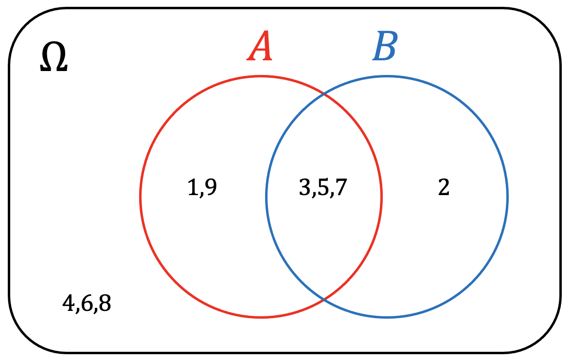
If we were to sample one element, probabilities can be formalized using combinatorics:

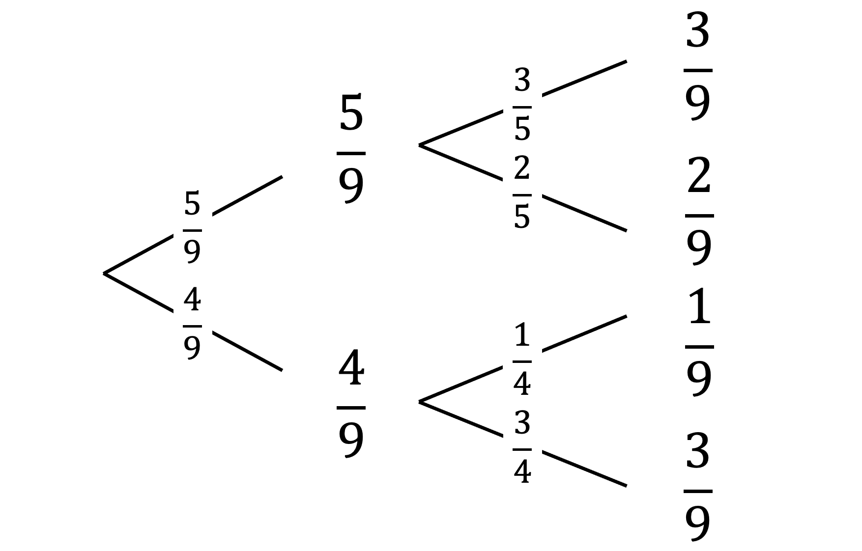
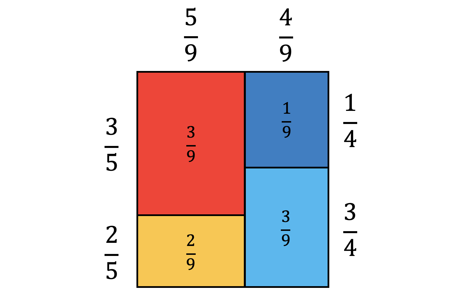
\[\begin{equation} P ( A ) = \frac{ C_{1}^{5} }{ C_{1}^{9} } = \frac{5}{9} \qquad P ( A' ) = \frac{ C_{1}^{4} }{ C_{1}^{9} } = \frac{4}{9} \qquad P ( A \vert B ) = \frac{ C_{1}^{3} }{ C_{1}^{4} } = \frac{3}{4} \\ P ( A \cup B ) = \frac{ C_{1}^{6} }{ C_{1}^{9} } = \frac{6}{9} \qquad P ( A \cap B ) = \frac{ C_{1}^{3} }{ C_{1}^{9} } = \frac{3}{9} \qquad P ( A' \cap B' ) = \frac{ C_{1}^{3} }{ C_{1}^{9} } = \frac{3}{9} \end{equation}\]

Furthermore, they can be intuitively visualized as:

Venn diagram	Tree diagram	Square diagram

The above problems deal with a single sample. If we were to sample two items without replacements, there exist two probability spaces, before and after sampling the first element. Consider $E_{AB} E_{AB}$ as sampling two elements that are both odd and prime and $E_{A} E_{AB}$ as sampling one odd non-prime number and another odd prime number.

\[\begin{align} P ( E_{AB} E_{AB} ) & = \frac{ C_{2}^{3} }{ C_{2}^{9} } = \frac{ C_{1}^{3} }{ C_{1}^{9} } \cdot \frac{ C_{1}^{2} }{ C_{1}^{8} } = \frac{1}{12} \\ P ( E_{A} E_{AB} ) & = \frac{ C_{1}^{2} \cdot C_{1}^{3} }{ C_{2}^{9} } = \frac{ C_{1}^{2} }{ C_{1}^{9} } \cdot \frac{ C_{1}^{3} }{ C_{1}^{8} } + \frac{ C_{1}^{3} }{ C_{1}^{9} } \cdot \frac{ C_{1}^{2} }{ C_{1}^{8} } = \frac{1}{6} \end{align}\]

Sampling one element without replacements reduces the size of the set from $9$ to $8$ for sampling the second element. Visualizing this requires two diagrams, one for the set with the size of $9$ before the first sampling, which is shown above, and the other for the set with the size of $8$ after the first sampling.

Statistics

Statistics deals with the collection, analysis, interpretation, and presentation of data. It extracts information from data and draws conclusions about the population. It is important for making data-driven decisions, testing hypotheses, and understanding patterns and trends in data.

Population and Sample

Statistics is all about data. The terms used in statistics differ from probability.

A set in probability is a dataset in statistics.
An element in the set in probability is an observation or value in the dataset in statistics.
An independent and identically distribution (IID) in probability is a random sampling in statistics.

In statistics, a dataset is divided into two concepts.

A population refers to the entire group of observation that meet a specific set of criteria and are of interest.
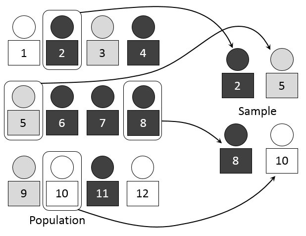
A sample refers to a subset of a population that is selected to be used to estimate the characteristics of the population.

Using a population is ideal, but it is often impractical or impossible to collect entire data on the study of interest, and therefore, a sample is often acquired using sampling techniques to represent the population.

A visual representation of sampling from Wikimedia Commons

There are two large classes of sampling technique.

Probability sampling sets known and non-zero probability of sampling to each observation from the population. Some common types are simple random sampling, systematic sampling, stratified sampling, and cluster sampling.
Non-probability sampling selects observations from the population based on convenience or priority. Some common types are convenience sampling, purposive or judgmental sampling, quota sampling, and snowball sampling.

Selecting the appropriate sampling technique depends on various factors, such as the purpose and availability.

Therefore, statistics is said to be the discipline that attempts to draw conclusions of the population of interest by analyzing a sample acquired from the population using sampling.

Statistical Analysis

Statistical analysis is to identify patterns, relationships, or trends that may be present in the data. There are two categories in statistical analysis, descriptive statistics and inferential statistics.

A population is defined as a collection of $N$ observations of $x_{i}$, where each observation may appear more than once. A sample, on the other hand, is a subset of the population consisting of $n$ observations of $x_{i}$.

Descriptive statistics is to summarize the characteristics of a data, i.e. mean and standard deviation.
- Measurements of the central tendency can be divided into:
  - Mean ($\mu$): The average value of the data, $\mu = \frac{ \sum_{i = 1}^{N} x_{i} }{ N }$.
  - Median: The middle value of the data, where if the data size is an even number, the median is the average of the two middle values.
  - Mode: The most frequently appeared value of the data, where if there are two or more values that occur with the same frequency, then the data is said to have multiple modes.
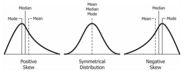
  The difference between mean, median and mode from Wikimedia Commons
- Measurements of the dispersion can be divided into:
  - Standard deviation ($\sigma$): The average squared distance of values from the mean, $\sigma = \sqrt{ \frac{ \sum_{i = 1}^{N} ( x_{i} - \mu )^{2} }{ N } }$.
  - Interquartile range (IQR): The range between the 25th and 75th percentiles of the data, where if the data size is an even number, it is the average of the two values.
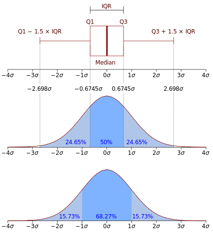
  The difference between standard deviation and IQR from Wikimedia Commons

Inferential statistics is to make predictions or draw conclusions about data, i.e. hypothesis testing and estimation.

Hypothesis testing, or statistical hypothesis testing, is a method to decide if a particular hypothesis about a population can be sufficiently supported with a sample.

Define a null hypothesis ($H_{0}$) that you will reject if the hypothesis testing is True. This is what you do not want to support.
Define an alternative hypothesis ($H_{a}$) that you will accept if the hypothesis testing is True. This is what you want to support.
Determine and calculate an appropriate test statistic and its associated probability.
If the probability is small, reject $H_{0}$ and accept $H_{a}$, otherwise, accept $H_{0}$ and reject $H_{a}$.

Error Types		$ H_{0} $ is
Error Types		True	False
Hypothesis Testing on $ H_{0} $	Accept	Correct Inference (True Negative)	Type II Error (True Negative)
Hypothesis Testing on $ H_{0} $	Reject	Type I Error (False Positive)	Correct Inference (True Positive)

Statistical estimation is a method of estimating the quantity of interest based on observed data. The simplest estimation technique is point estimation, which computes a single value, referred to as a point estimate, that serves as an estimated value of an unknown population parameter.
- Sample mean, $\bar{x} = \frac{ \sum_{i = 1}^{n} x_{i} }{ n }$, is said to be a point estimate for population mean ($\mu$). In other words, $\mu$ is an estimand and $\bar{x}$ is an estimator of $\mu$.
- Sample standard deviation, $s = \sqrt{ \frac{ \sum_{i = 1}^{n} ( x_{i} - \bar{x} )^{2} }{ n - 1 } }$, is said to be a point estimate for population standard deviation ($\sigma$). In other words, $\sigma$ is an estimand and $s$ is an estimator of $\sigma$.

Bias

Bias is a systematic error or distortion, deviating from the true value. It is a typical problem in statistics when collecting or analyzing data.

Sample data may carry bias from three sources:

Data is measured incorrectly. This may be due to observation errors, instrumental errors, environmental errors and many more.
Sampling is inappropriate for the desired conclusion. For instance, those what are sold in the market in specific regions can only be used to study the trends of popular products within those selected regions, not within the country.
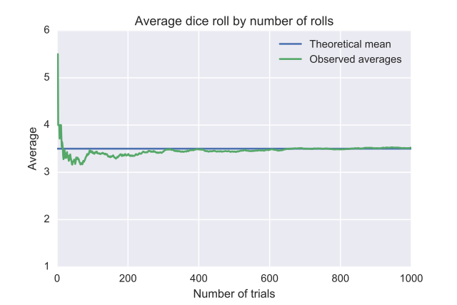
The sample size is too small. Small number of observation may introduce bias even with the correct data measurement and sampling technique. This phenomenon is referred to as the law of large number, which means that as the sample size grows, the estimated value becomes closer to the true value, i.e. average.

Average dice roll by the number of rolls from Wikimedia Commons

On the other hand, population data may carry bias from only one source, incorrect data measurement. If the observation is measured correctly, the results acquired from statistical analysis upon the population data is the true value.

While mean is the same between sample and population, standard deviation is different between them.

\[\begin{equation} \sigma = \sqrt{ \frac{ \sum_{i = 1}^{N} ( x_{i} - \mu )^{2} }{ \color{red}{N} } } \qquad s = \sqrt{ \frac{ \sum_{i = 1}^{n} ( x_{i} - \bar{x} )^{2} }{ \color{red}{n - 1} } } \end{equation}\]

$s$ uses a denominator of $n - 1$ instead of $n$ to correct bias that may potentially have been introduced from low sample size. As a result, $s$ tends to be slightly larger than $\sigma$, especially when $n$ is small.

Define single digit positive integers to be population, that is a set, $S = \{ 1 , 2 , 3 , 4 , 5 , 6 , 7 , 8 , 9 \}$, where $N = 9$. Population standard deviation is:

\[\begin{align} \sigma & = \sqrt{ \frac{ \sum_{x_{i} \in S} ( x_{i} - \mu )^{2} }{ N } } \quad \mu = \frac{ \sum_{x_{i} \in S} x_{i} }{ N } = \frac{ \sum_{i = 1}^{9} i }{ 9 } = 5 \\ & = \sqrt{ \frac{ \sum_{i = 1}^{9} ( i - 5 )^{2} }{ 9 } } = \sqrt{ \frac{ 60 }{ 9 } } = 2.5820 \end{align}\]

If we were to sample $n$ number of observations, the average value of sample standard deviation and population standard deviation are:

\[\begin{equation} \bar{\sigma}_{n=2} = 1.6667 \qquad \bar{s}_{n=2} = 2.3570 \qquad \bar{\sigma}_{n=3} = 2.1074 \qquad \bar{s}_{n=3} = 2.5810 \end{equation}\]

Bias used in mathematics has slight difference with bias in psychology. Psychological bias refers to a tendency to think or act in a way that is influenced by unconscious factors such as emotions, beliefs, or past experiences. However, even in the world of psychology, the interpretation behind bias is different between people. Some people consider bias as errors to avoid, same as bias in mathematics, while others view it as a natural concept for evolution and pattern recognition, for instance, how we form bias towards lions eating gazelles or supermarkets stocking eggs. Nevertheless, in mathematics, bias is considered as errors of the estimated value deviated from the true value.

Also note that in statistical modelling, bias can also be arisen from model itself, not from data. This bias is used in bias-variance trade-off.

Markov Model

A Markov model is a stochastic process that describes pseudo-randomly changing systems under the Markov property, or the Markov assumption. The Markov property stipulates the future state depends only on the current state, not the history of states. There are four common Markov models:

	Fully Observable	Partially Observable
Autonomous System	Markov Chain	Hidden Markov Model
Controllable System	Markov Decision Process	Partially Observable Markov Decision Process

Mathematics

D. K. Ryu