Markov Chain
Prerequisites
- Basic probability
All is number.
Pythagoras
Humans have invented and developed languages to symbolize entities, constructing Matrix that captures the essence of reality. On the other hand, any form of entities can be modelled as number, from natural to complex numbers and from points to objects, which existed long before human civilization. Thereby, the universe itself is inherently number, or in short, all is number.
Mathematics is the study of numbers, so if an entity exists, there exists mathematics to describe it, even if we cannot perceive. This is why we (arguably) refer mathematics as discovery instead of invention and often considered the most fundamental and precise way of describing reality. Mathematics is a vast, diverse and abstract field such that it requires books of worth. Here, a few branches of mathematics are focused on.
A Markov model is a stochastic process that describes pseudo-randomly changing systems under the Markov property, or the Markov assumption. The Markov property stipulates the future state depends only on the current state, not the history of states. There are four common Markov models:
| Fully Observable | Partially Observable | |
| Autonomous System | Markov Chain | Hidden Markov Model |
| Controllable System | Markov Decision Process | Partially Observable Markov Decision Process |
A Markov chain is the simplest form of a Markov model, which describes the world with an autonomous system. It is used to model simulations, speech recognition, time series forecasting, bioinformatics, game theories and many more. This post aims to provide a tutorial on a Markov chain and introduce a commonly used variant, a hidden Markov model.
Markov Chain
A Markov chain (MC), or Markov process, is the simplest form of a Markov model. In an MC, there exists a system that starts at a particular state, and every time step, the system travels to neighbouring states within the MC.
The Markov property is formally defined as following. There exists a state, \(s \in \mathcal{S}\), and a transition probability, \(p \in \mathcal{P}\), such that:
\[\begin{equation} \Pr ( S_{t+1} = s_{t+1} \vert S_{0:t} = s_{0:t} ) \equiv p ( S_{t+1} = s_{t+1} \vert S_{t} = s_{t} ) = p ( s_{t+1} \vert s_{t} ) \end{equation}\]Where \(S_{0:t} = s_{0:t}\) signifies a sequence of states that the system visits from \(0\) to \(t\) time, \(S_{0} = s_{0} , \cdots , S_{t} = s_{t}\). A collection of states that the system visited for a given maximum time, \(T\), is referred to as a path, \(\{ S_{0} = s_{0} , \cdots S_{T} = s_{T} \}\). Unlike computer science, people from mathematics often refer to a state as an event or a process with \(\{ X_{t} \}_{t=0}^{T}\) notation.
The Markov property assumes that the probability of transitioning between two states is only dependent on the one-step previously visited states, not on the history of all the previously visited states. This allows us to formalize the transition probabilities as a fixed transition matrix, \(\mathbf{P}\):
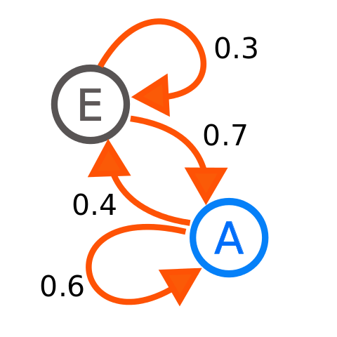
\[\begin{equation} \mathbf{P} = \begin{bmatrix} p ( s_{1} \vert s_{1} ) & p ( s_{2} \vert s_{1} ) & \cdots & p ( s_{n} \vert s_{1} ) \\ p ( s_{1} \vert s_{2} ) & p ( s_{2} \vert s_{2} ) & \cdots & p ( s_{n} \vert s_{2} ) \\ \vdots & \vdots & \ddots & \vdots \\ p ( s_{1} \vert s_{n} ) & p ( s_{2} \vert s_{n} ) & \cdots & p ( s_{n} \vert s_{n} ) \\ \end{bmatrix} \end{equation}\]Consider the following MC.
| Example Markov Chain from Wikimedia Commons | |
|
$$ \begin{align} \mathbf{P} & = \begin{bmatrix} p ( E \vert E ) & p ( A \vert E ) \\ p ( E \vert A ) & p ( A \vert A ) \\ \end{bmatrix} \\ & = \begin{bmatrix} 0.3 & 0.7 \\ 0.4 & 0.6 \\ \end{bmatrix} \end{align} $$ |
\(\mathbf{P}\) is what determines the property of a state in an MC, and moreover, the property of an MC. However, \(\mathbf{P}\) is not really intuitive, so instead, we usually analyze the accessibility of states from each other, referred to as communication.
- If \(s_{i}\) communicates with itself, \(s_{i} \leftrightarrow s_{i}\).
- If \(s_{i}\) communicates with \(s_{j}\), \(s_{i} \leftrightarrow s_{j}\).
- If \(s_{i}\) communicates with \(s_{k}\) through \(s_{j}\), \(s_{i} \leftrightarrow s_{j}\) and \(s_{j} \leftrightarrow s_{k}\), then \(s_{i} \leftrightarrow s_{k}\).
With these, we can determine the property of an MC. Few additional important concepts in an MC are:
- A closed set is a set of states that the system cannot entre or leave.
- A set includes a single element as well, so a state alone can be a closed set.
- An initial distribution is a probability distribution over states that the system starts. It is a row vector, \(\pi^{(0)} \in \mathbb{R}^{n}\).
- The proability of the system visiting states at \(k\) step for a given \(\pi^{(0)}\) is \(\pi^{(0)} \mathbf{P}^{k}\).
- A stationary distribution is an equilibrium probability distribution over states that do not change over time. It is a row vector, \(\pi \in \mathbb{R}^{n}\).
- \(\pi\) is the left eigenvector for \(\mathbf{P}\), or \(\pi = \pi \mathbf{P}\).
- There may exist more than one \(\pi\) depending on the perperty of an MC.
- A limiting distribution is a unique non-zero equilibrium probability distribution over states that the system will end up if it travels infinitely. It is a row vector, \(\pi^{(\infty)} \in \mathbb{R}^{n}\).
- \(\pi^{(\infty)}\) is the proability of the system visiting states at an infinite step for a given \(\pi^{(0)}\), or \(\pi^{(\infty)} = \pi^{(0)} \mathbf{P}^{\infty}\).
- Similar to \(\pi\), \(\pi^{(\infty)}\) is the left eigenvector for \(\mathbf{P}\), or \(\pi^{(\infty)} = \pi^{(\infty)} \mathbf{P}\).
- Unlike \(\pi^{(0)}\) and \(\pi\), \(\pi^{(\infty)}\) may not exist depending on the property of an MC. If \(\pi^{(\infty)}\) exists, it is unique and equivalent to \(\pi\), or \(\pi^{(\infty)} = \pi\).
- In other words, if \(\pi^{(\infty)}\) exists, there only exists a single \(\pi\) such that \(\pi = \pi^{(\infty)}\).
Usually, \(\mathbf{P}\) is used to determine:
- Whether a particular state communicates with other states.
- The characteristics of the stationary distribution.
- The existence of the limiting distribution.
Here, I will go through some typical properties of states and MC, particularly about countably finite discrete-time MC.
Absorption
A state is referred to as an absorbing state and a chain of states is referred to as an absorbing chain if the system cannot leave once entered, or absorption occurs. An MC with an absorbing state and/or an absorbing chain is referred to as an absorbing MC. In an absorbing MC, a non-absorbing state is referred to as a transient state. Thus, two types of states exist, absorbing and transient in an absorbing MC.
In an absorbing MC, \(\mathbf{P} \in \mathbb{R}^{n \times n}\) is usually expressed in canonical form. Let \(t\) be transient states and \(r\) be absorbing states, where \(n = t + r\).
\[\begin{equation} \mathbf{P} = \begin{bmatrix} \mathbf{Q} & \mathbf{R} \\ \mathbf{0} & \mathbf{I} \\ \end{bmatrix} \end{equation}\]- \(\mathbf{Q} \in \mathbb{R}^{t \times t}\) is \(p\) between transient states.
- \(\mathbf{R} \in \mathbb{R}^{t \times r}\) is \(p\) from transient states to absorbing states.
- \(\mathbf{I} \in \mathbb{R}^{r \times r}\) is \(p\) between absorbing states.
- \(\mathbf{0} \in \mathbb{R}^{r \times t}\) is \(p\) from absorbing states to transient states, which is \(0\)-matrix.
A fundamental matrix, \(\mathbf{N} \in \mathbb{R}^{t \times t}\), is the expected number of the visitations between every transient state before absorption, \(\mathbf{N} = \sum_{k=0}^{\infty} \mathbf{Q}^{k} = ( \mathbf{I} - \mathbf{Q} )^{-1}\).
- Each \(( i , j )\) element represents the expected number of the visitations from \(s_{i}\) to \(s_{j}\) before absorption.
- \(\mathbf{Q}^{k}\) is the proability of the system travelling between transient states at \(k\) step.
- \(\mathbf{Q}^{\infty}\) approaches zero over time, \(\lim_{ k \rightarrow \infty } \mathbf{Q}^{k} = \mathbf{0} \in \mathbb{R}^{t \times t}\).
- Under the Taylor series, \(\frac{1}{1-x} = \sum_{k=0}^{\infty} x^{k}\), and thus, \(\frac{1}{\mathbf{I} - \mathbf{Q}} = ( \mathbf{I} - \mathbf{Q} )^{-1} = \sum_{k=0}^{\infty} \mathbf{Q}^{k} = \mathbf{N}\).
An irreduciblility is another commonly seen term in an absorbing MC. It is often confused with absorption since it can be a synonym or antonym based on the context. A set of states that the system cannot leave once entered is referred to as a closed irreducible set. An MC with a closed irreducible set is referred to as a reducible MC.
Thus, a closed irreducible set is a synonym for an absorbing state and absorbing chain, but an absorbing MC is antonym for an irreducible MC. More formally:
- An MC is an absorbing MC if there exist one or more closed irreducible sets, in which the system can reach from any state in a finite number of steps.
- An MC is an irreducible MC if the system can reach any state from any other state in a finite number of time step.
If an absorbing MC is reduced into multiple disjoint subsets based on reduciblility, that are an absorbing state, an absorbing chain and a chain of transient states, states in each subset has the property that all states can communicate with each other, i.e. absorbing or transient.
Recurrence
A state is referred to as a recurrent state if the system is guaranteed to return to the starting state within a finite step. Note that the term recurrent is not often used to refer to an MC. More formally, a state is a recurrent state if:
\[\begin{equation} \sum_{t = 1}^{\infty} \Pr ( S_{t} = s_{i} \vert S_{0} = s_{i} ) = 1 \end{equation}\]- \(\Pr ( S_{t} = s_{i} \vert S_{0} = s_{i} )\): For a given starting state, \(s_{i}\), the probability of the system returning to \(s_{i}\) at \(t\) step.
- \(\sum_{t = 1}^{\infty} \Pr ( S_{t} = s_{i} \vert S_{0} = s_{i} ) = 1\): The sum of the probabilities that the system will return to \(s_{i}\) is \(1\) in finite step. This means that the system guarantees that it will re-visit the starting state.
- The notation omits \(S_{1} \neq s_{i} , \cdots , S_{t-1} \neq s_{i}\), so what it really signifies is \(\Pr ( S_{t} = s_{i} \vert S_{0} = s_{i} , S_{1} \neq s_{i} , \cdots , S_{t-1} \neq s_{i} )\). This means that, for a given \(S_{0} = s_{i}\), the probability of the system returning to \(s_{i}\) at \(t\) step without visiting \(s_{i}\) in between.
This definition is equivalent to all the following statements:
- \(\sum_{t=1}^{\infty} \mathbb{1} ( S_{t} = s_{i} \vert S_{0} = s_{i} ) = \infty\): For a given \(S_{0} = s_{i}\), the summation of the booleans that the system will return to \(s_{i}\) is infinite.
- \(\mathbb{1} ( S_{t} = s_{i} \text{ for infinitely many } t \vert S_{0} = s ) = 1\): For a given \(S_{0} = s_{i}\), the boolean that the system will return to \(s_{i}\) for infinitely many \(t\) is 1.
If the system is not guaranteed to return, the state is referred to as a transient state, which is equivalent to the transient in an absorbing MC. More formally:
\[\begin{equation} \sum_{t=1}^{\infty} \Pr ( S_{t} = s_{i} \vert S_{0} = s_{i} ) < 1 \\ \sum_{t=1}^{\infty} \mathbb{1} ( S_{t} = s_{i} \vert S_{0} = s_{i} ) < \infty \\ \mathbb{1} ( S_{t} = s_{i} \text{ for infinitely many } t \vert S_{0} = s_{i} ) = 0 \end{equation}\]An absorbing MC is the common MC that contains both recurrent and transient states.
- An absorbing state is the recurrent state. If \(s_{i}\) is absorbing, \(\Pr ( S_{1} = s_{i} \vert S_{0} = s_{i} ) = 1\) and \(\Pr ( S_{n} = s_{i} \vert S_{0} = s_{i} ) = 0\) for \(n > 1\).
- All the states in an absorbing chain is the recurrent states. If \(s_{i}\) is within the absorbing chain, \(\sum_{t = 1}^{\infty} \Pr ( S_{t} = s_{i} \vert S_{0} = s_{i} ) = 1\) within the absorbing chain.
- A non-absorbing state is the transient state. If \(s_{i}\) is not absorbing, the system will fall into an absorbing state or chain within a finite step, \(\sum_{t=1}^{\infty} \Pr ( S_{t} = s_{i} \vert S_{0} = s_{i} ) < 1\).
A recurrence is to claim that the system will return to the starting state. However, there is a further division, positive or null. Both of them guarantee that the system will return to the starting state, but what matters is when. More formally, let a hitting time to be \(\tau_{s} := \inf \{ t \geq 0 : s_{i} \in \mathcal{S} \}\), which is the infimum of the number of steps that the system returns to the starting state, \(s_{i}\).
- Positive Recurrent: \(\tau_{s}\) is finite and finite expectation, or \(\tau_{s} < \infty\) and \(\mathbb{E} \left[ \tau_{s} \right] < \infty\), and thus, guaranteed to return in finite step.
- Null Recurrent: \(\tau_{s}\) is finite, but infinite expectation, or \(\tau_{s} < \infty\) and \(\mathbb{E} \left[ \tau_{s} \right] = \infty\), and thus, guaranteed to return in infinite step.
- Transient: \(\tau_{s}\) is infinite and infinite expectation, or \(\tau_{s} = \infty\) and \(\mathbb{E} \left[ \tau_{s} \right] = \infty\), and thus, not guaranteed to return.
Due to this, positive recurrent is often described as it will return in a finite step while null recurrent as it will almost certainly return in a finite step.
A null recurrent state can only be present in a countably infinite MC, so in a countably finite MC, if an MC is said to be recurrent, it is always positive recurrent.
- If an MC is countably finite:
- There must be at least one recurrent state.
- If reducible, an absorbing state or chain is recurrent and others are transient.
- If irreducible, every state is positive recurrent.
- There can be no transient state, but not every state can be transient.
- There must be at least one recurrent state.
- If an MC is countably infinite:
- Every state can be either positive recurrent, null recurrent or transient.
Periodicity
A state is referred to as a periodic state if the system returns to a particular state \(s_{i}\) at some rates \(\{ n , 2n , 3n , \cdots \}\), where \(n > 1\). For instance, for a given \(S_{0} = s_{i}\), if the system returns to \(s_{i}\) at \(t = \{ 4 , 16 , 24 , 28 , \cdots \}\), then the state is periodic with \(n = 4\). If one state is periodic, then all the other states are periodic with the same period \(n\). An MC with periodic states is referred to as a periodic MC.
If at least one state has \(p\) to itself, \(p ( s_{i} \vert s_{i} ) > 0\), the state is aperiodic, and thus, the MC is also aperiodic. In general, it is said that an aperiodic MC has \(n = 1\) or \(n\) does not exist.
To compare with other properties:
- If an MC is absorbing, it cannot be periodic since the system will get stuck at an absorbing state or chain in a finite step.
- If an MC is transient or null recurrent, it cannot be periodic since the system may never return or return in an infinite step.
- Thus, a periodic MC is always irreducible and positive recurrent while aperiodic can hold any property. However, irreducible and/or positive recurrent does not tell us any information about periodicity.
Ergodicity
The ergodicity is one of the typical assumptions in an MC for machine learning applications. It is derived from ergodic theory, a branch of mathematics that studies statistical properties of deterministic dynamical systems, but the use of ergodicity is fairly simple in machine learning. The regular MC we usually refer to in machine learning actually refers to an ergodic MC.
An MC is referred to as an ergodic MC if the system can travel from any state to any other state in any period, a.k.a. aperiodic, irreducible and positive recurrent. If an MC is ergodic, there exists a limiting distribution.
\[\begin{equation} \pi_{i}^{(\infty)} = \lim_{n \rightarrow \infty} \Pr ( S_{n} = s_{i} \vert S_{0} = s ) > 0 \quad s \in \mathcal{S} \end{equation}\]This means, given any starting state, there exists a unique non-zero equilibrium probability that the system lands on a particular state, regardless of where it starts, if it travels infinitely.
A limiting distribution is often interchangeably used with a stationary distribution, but they are different.
- A stationary distribution is an equilibrium probability distribution that does not change over time, which is the left eigenvector for \(\mathbf{P}\), \(\pi = \pi \mathbf{P}\), such that \(\pi_{i} \geq 0 , \sum_{i}^{n} \pi_{i} = 1\), where \(\mathcal{S} = \{ s_{0} , \cdots , s_{n} \}\).
- For an MC to have \(\pi\), it must have at least one positive recurrent state, in other words, if an MC has countably finite states, it has \(\pi\).
- There is no restriction on how many \(\pi\) to exist, and thus, there may be more than one \(\pi\).
- For instance, a periodic MC has a single \(\pi\) while an absorbing MC has infinitely many \(\pi\).
- One way to obtain \(\pi\) is by finding eigenvalues and eigenvectors of the transposed \(\mathbf{P}\).
- However, this method does not obtain every \(\pi\). For instance, in an absorbing MC, there are infinitely many \(\pi\) and this method only acquires a few instances.
-
Another way to view \(\pi\) is from \(\tau_{s}\).
\[\begin{equation} \pi_{i} = \frac{1}{ \mathbb{E} \left[ \tau_{i} \right] } \end{equation}\]- This also reflects why if \(\mathbb{E} \left[ \tau_{s} \right] = \infty\), i.e. null recurrent or transient, \(\pi\) approaches zero.
- For an MC with null recurrent states only or transient states only, \(\tau_{s}\) for all the states is infinite, so \(\sum_{i}^{\infty} \pi_{i} = 1\) does not hold, and thus, there is no \(\pi\). Often determining if a \(\pi\) exists in the case of a recurrent MC is a method of proving if an MC is positive recurrent.
- So, if an MC is countably finite, at least one \(\pi\) exists, but if countably infinite, there may be no \(\pi\).
- A limiting distribution is a unique non-zero equilibrium distribution that is not dependent on an initial distribution, \(\pi_{i}^{(\infty)} = \lim_{n \rightarrow \infty} \Pr ( S_{n} = s_{i} \vert S_{0} = s ) > 0\).
- Since \(\pi^{(\infty)}\) is a unique distribution, the multiplication of \(\mathbf{P}\) to any \(\pi^{(0)}\) converges to \(\pi^{(\infty)}\).
- A periodic MC has no \(\pi^{(\infty)}\) since it oscillates periodically.
- An absorbing MC has no \(\pi^{(\infty)}\) since it converges to a distribution dependent to \(\pi^{(0)}\) and the converged distribution contains zero value at transient states.
- If \(\pi^{(\infty)}\) exists, \(\pi^{(\infty)} = \pi\), and thus, \(\pi\) is non-zero and unique.
Therefore:
- The existence of \(\pi^{(\infty)}\) is necessary and sufficient for the ergodicity of an MC.
- The ergodicity of an MC is necessary and sufficient for the existence of \(\pi^{(\infty)}\).
- The existence of \(\pi^{(\infty)}\) is only sufficient for a non-zero unique \(\pi\), not necessary.
- A non-zero unique \(\pi\) is neither necessary nor sufficient for the existence of \(\pi^{(\infty)}\).
- A non-zero unique \(\pi\) is neither necessary nor sufficient for the ergodicity of an MC.
Markov Chain Example
To give better insights, I will go through some examples.
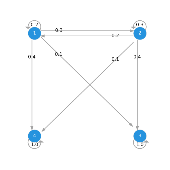
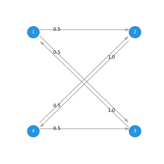
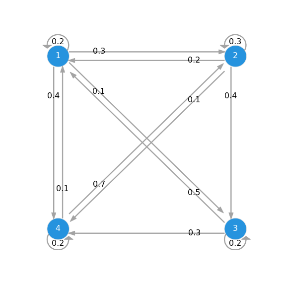
| Absorbing Markov chain | Periodic Markov chain | Ergodic Markov chain |
|
|
|
| $ 1 $ and $ 2 $ are transient while $ 3 $ and $ 4 $ are absorbing. | All are periodic with $ n = 2 $, $ \{ 2, 4, 6, \cdots \} $. | Other than $ p ( 3 \vert 4 ) $ and $ p ( 2 \vert 3 ) $, all the transition probabilities are non-zero. |
| $$ \begin{equation} \mathbf{P} = \begin{bmatrix} 0.2 & 0.3 & 0.1 & 0.4 \\ 0.2 & 0.3 & 0.4 & 0.1 \\ 0.0 & 0.0 & 1.0 & 0.0 \\ 0.0 & 0.0 & 0.0 & 1.0 \\ \end{bmatrix} \end{equation} $$ | $$ \begin{equation} \mathbf{P} = \begin{bmatrix} 0.0 & 0.5 & 0.5 & 0.0 \\ 0.0 & 0.0 & 0.0 & 1.0 \\ 1.0 & 0.0 & 0.0 & 0.0 \\ 0.0 & 0.5 & 0.5 & 0.0 \\ \end{bmatrix} \end{equation} $$ | $$ \begin{equation} \mathbf{P} = \begin{bmatrix} 0.2 & 0.3 & 0.1 & 0.4 \\ 0.2 & 0.3 & 0.4 & 0.1 \\ 0.5 & 0.0 & 0.2 & 0.3 \\ 0.1 & 0.7 & 0.0 & 0.2 \\ \end{bmatrix} \end{equation} $$ |
Absorbing Markov Chain
An absorbing MC has infinitely many stationary distributions, but no limiting distribution. The eigenvalues and eigenvectors for \(\mathbf{P}^{\intercal}\) are:
\[\begin{equation} \lambda \pi^{\intercal} = \mathbf{P}^{\intercal} \pi^{\intercal} \quad \rightarrow \quad \pi = \begin{bmatrix} 0.0 & 0.0 & 1.0 & 0.0 \\ \end{bmatrix} \quad \text{or} \quad \begin{bmatrix} 0.0 & 0.0 & 0.0 & 1.0 \\ \end{bmatrix} \end{equation}\]However, they are not all. Consider the transition matrix.
\[\begin{equation} \mathbf{P} = \begin{bmatrix} 0.2 & 0.3 & 0.1 & 0.4 \\ 0.2 & 0.3 & 0.4 & 0.1 \\ 0.0 & 0.0 & 1.0 & 0.0 \\ 0.0 & 0.0 & 0.0 & 1.0 \\ \end{bmatrix} \quad \rightarrow \quad \mathbf{P}^{\infty} = \begin{bmatrix} 0.0 & 0.0 & 0.38 & 0.62 \\ 0.0 & 0.0 & 0.68 & 0.32 \\ 0.0 & 0.0 & 1.0 & 0.0 \\ 0.0 & 0.0 & 1.0 & 0.0 \\ \end{bmatrix} \end{equation}\]Under different initial distributions:
\[\begin{align} \pi^{(0)} = \begin{bmatrix} 1.0 & 0.0 & 0.0 & 0.0 \\ \end{bmatrix} \quad \rightarrow \quad & \pi^{(\infty)} = \pi^{(0)} \mathbf{P}^{\infty} = \begin{bmatrix} 0.0 & 0.0 & 0.38 & 0.62 \\ \end{bmatrix} \\ \pi^{(0)} = \begin{bmatrix} 0.2 & 0.8 & 0.0 & 0.0 \\ \end{bmatrix} \quad \rightarrow \quad & \pi^{(\infty)} = \pi^{(0)} \mathbf{P}^{\infty} = \begin{bmatrix} 0.0 & 0.0 & 0.62 & 0.38 \\ \end{bmatrix} \\ \pi^{(0)} = \begin{bmatrix} 0.0 & 1.0 & 0.0 & 0.0 \\ \end{bmatrix} \quad \rightarrow \quad & \pi^{(\infty)} = \pi^{(0)} \mathbf{P}^{\infty} = \begin{bmatrix} 0.0 & 0.0 & 0.68 & 0.32 \\ \end{bmatrix} \\ \pi^{(0)} = \begin{bmatrix} 0.0 & 0.0 & 1.0 & 0.0 \\ \end{bmatrix} \quad \rightarrow \quad & \pi^{(\infty)} = \pi^{(0)} \mathbf{P}^{\infty} = \begin{bmatrix} 0.0 & 0.0 & 1.0 & 0.0 \\ \end{bmatrix} \\ \pi^{(0)} = \begin{bmatrix} 0.3 & 0.3 & 0.4 & 0.0 \\ \end{bmatrix} \quad \rightarrow \quad & \pi^{(\infty)} = \pi^{(0)} \mathbf{P}^{\infty} = \begin{bmatrix} 0.0 & 0.0 & 0.718 & 0.282 \\ \end{bmatrix} \end{align}\]- A stationary distribution depends on the initial distribution, so there is no unique equilibrium, a.k.a. no limiting distribution.
- Transient states always have zero stationary distribution, since the system falls into absorbing states.
- A fundamental matrix and an absorption time are:
- \(( i , j )\) element in \(\mathbf{Q}^{2}\) is the probability of visiting \(s_{j}\) from \(s_{i}\) at \(t = 2\), \(p ( S_{2} = s_{j} \vert S_{0} = s_{i}\).
- Every element in \(\mathbf{Q}^{\infty}\) reaches zero since the system falls into absorbing states.
- \(( i , j )\) element in \(\mathbf{N}\) is the number of times that the system will visit \(s_{j}\) from \(s_{i}\).
Periodic Markov Chain
A periodic MC has a single stationary distribution, but no limiting distribution since \(\lim_{k \rightarrow \infty} \mathbf{P}^{k}\) never converges.
\[\begin{equation} \lambda \pi^{\intercal} = \mathbf{P}^{\intercal} \pi^{\intercal} \quad \rightarrow \quad \pi = \begin{bmatrix} 0.25 & 0.25 & 0.25 & 0.25 \\ \end{bmatrix} \end{equation}\]For \(\mathbf{P}^{k}\), as \(k \rightarrow \infty\):
\[\begin{equation} \mathbf{P} = \begin{bmatrix} 0.0 & 0.5 & 0.5 & 0.0 \\ 0.0 & 0.0 & 0.0 & 1.0 \\ 1.0 & 0.0 & 0.0 & 0.0 \\ 0.0 & 0.5 & 0.5 & 0.0 \\ \end{bmatrix} \quad \mathbf{P}^{2} = \begin{bmatrix} 0.5 & 0.0 & 0.0 & 0.5 \\ 0.0 & 0.5 & 0.5 & 0.0 \\ 0.0 & 0.5 & 0.5 & 0.0 \\ 0.5 & 0.0 & 0.0 & 0.5 \\ \end{bmatrix} \\ \mathbf{P}^{3} = \begin{bmatrix} 0.0 & 0.5 & 0.5 & 0.0 \\ 0.5 & 0.0 & 0.0 & 0.5 \\ 0.5 & 0.0 & 0.0 & 0.5 \\ 0.0 & 0.5 & 0.5 & 0.0 \\ \end{bmatrix} \quad \mathbf{P}^{4} = \begin{bmatrix} 0.5 & 0.0 & 0.0 & 0.5 \\ 0.0 & 0.5 & 0.5 & 0.0 \\ 0.0 & 0.5 & 0.5 & 0.0 \\ 0.5 & 0.0 & 0.0 & 0.5 \\ \end{bmatrix} \end{equation}\]\(\mathbf{P}^{k}\) oscillates between \(\mathbf{P}^{2}\) and \(\mathbf{P}^{3}\), and thus,
\[\begin{equation} \pi^{(0)} = \begin{bmatrix} 1.0 & 0.0 & 0.0 & 0.0 \\ \end{bmatrix} \quad \pi^{(0)} \mathbf{P} = \begin{bmatrix} 0.0 & 0.5 & 0.5 & 0.0 \\ \end{bmatrix} \\ \pi^{(0)} \mathbf{P}^{2} = \begin{bmatrix} 0.5 & 0.0 & 0.0 & 0.5 \\ \end{bmatrix} \quad \pi^{(0)} \mathbf{P}^{3} = \begin{bmatrix} 0.0 & 0.5 & 0.5 & 0.0 \\ \end{bmatrix} \end{equation}\]So, it repeats between \(\begin{bmatrix} 0.5 & 0.0 & 0.0 & 0.5 \end{bmatrix}\) and \(\begin{bmatrix} 0.0 & 0.5 & 0.5 & 0.0 \end{bmatrix}\).
Ergodic Markov Chain
An ergodic MC has a limiting distribution, and so, a stationary distribution is unique.
\[\begin{align} \lambda \pi^{\intercal} = \mathbf{P}^{\intercal} \pi^{\intercal} \quad \rightarrow \quad & \pi = \begin{bmatrix} 0.236 & 0.334 & 0.197 & 0.233 \\ \end{bmatrix} \\ \mathbf{P} = \begin{bmatrix} 0.2 & 0.3 & 0.1 & 0.4 \\ 0.2 & 0.3 & 0.4 & 0.1 \\ 0.5 & 0.0 & 0.2 & 0.3 \\ 0.1 & 0.7 & 0.0 & 0.2 \\ \end{bmatrix} \quad \rightarrow \quad & \mathbf{P}^{\infty} = \begin{bmatrix} 0.236 & 0.334 & 0.197 & 0.233 \\ 0.236 & 0.334 & 0.197 & 0.233 \\ 0.236 & 0.334 & 0.197 & 0.233 \\ 0.236 & 0.334 & 0.197 & 0.233 \\ \end{bmatrix} = \begin{bmatrix} \pi \\ \pi \\ \pi \\ \pi \\ \end{bmatrix} \end{align}\]Under different initial distributions:
\[\begin{align} \pi^{(0)} = \begin{bmatrix} 1.0 & 0.0 & 0.0 & 0.0 \\ \end{bmatrix} \quad \rightarrow \quad & \pi^{(\infty)} = \pi^{(0)} \mathbf{P}^{\infty} = \begin{bmatrix} 0.236 & 0.334 & 0.197 & 0.233 \\ \end{bmatrix} = \pi \\ \pi^{(0)} = \begin{bmatrix} 0.2 & 0.8 & 0.0 & 0.0 \\ \end{bmatrix} \quad \rightarrow \quad & \pi^{(\infty)} = \pi^{(0)} \mathbf{P}^{\infty} = \begin{bmatrix} 0.236 & 0.334 & 0.197 & 0.233 \\ \end{bmatrix} = \pi \\ \pi^{(0)} = \begin{bmatrix} 0.0 & 1.0 & 0.0 & 0.0 \\ \end{bmatrix} \quad \rightarrow \quad & \pi^{(\infty)} = \pi^{(0)} \mathbf{P}^{\infty} = \begin{bmatrix} 0.236 & 0.334 & 0.197 & 0.233 \\ \end{bmatrix} = \pi \end{align}\]So, the stationary distribution converges the same regardless of the initial distribution, and hence, it is the limiting distribution.
Hidden Markov Model
A hidden Markov model (HMM) is an MC with partial observability. The idea behind an HMM is that the state is hidden from the system, or a hidden state or unobserved event or latent variable. So, instead of observing a state, the system needs to infer the state from an additional variable, referred to as an observation, \(\mathcal{O}\). There also exists a probability of emitting different observations for a given state, referred to as an emission probability, \(\mathcal{P}_{o}\).
An emission probability also holds the Markov property. There exists an observation, \(o \in \mathcal{O}\), and an emission probability, \(p_{o} \in \mathcal{P}_{o}\), such that,
\[\begin{equation} \Pr ( O_{t} = o_{t} \vert S_{1:t} = s_{1:t} , O_{1:t-1} = o_{1:t-1} ) \equiv p_{o} ( O_{t} = o_{t} \vert S_{t} = s_{t} ) = p_{o} ( o_{t} \vert s_{t} ) \end{equation}\]So, in an HMM, \(p\) and \(p_{o}\) are only dependent on the previous state and the current state, respectively.
Consider the following HMM.
| Hidden Markov model from Wikimedia Commons | |
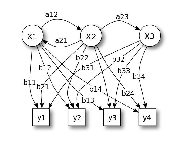
|
$$ \begin{equation} \mathbf{P} = \begin{bmatrix} p ( X1 \vert X1 ) & p ( X2 \vert X1 ) & p ( X3 \vert X1 ) \\ p ( X1 \vert X2 ) & p ( X2 \vert X2 ) & p ( X3 \vert X2 ) \\ p ( X1 \vert X3 ) & p ( X2 \vert X3 ) & p ( X3 \vert X3 ) \\ \end{bmatrix} \\ \mathbf{P}_{o} = \begin{bmatrix} p ( y1 \vert X1 ) & p ( y2 \vert X1 ) & p ( y3 \vert X1 ) & p ( y4 \vert X1 ) \\ p ( y1 \vert X2 ) & p ( y2 \vert X2 ) & p ( y3 \vert X2 ) & p ( y4 \vert X2 ) \\ p ( y1 \vert X3 ) & p ( y2 \vert X3 ) & p ( y3 \vert X3 ) & p ( y4 \vert X3 ) \\ \end{bmatrix} \end{equation} $$ |
The joint probability of all the states and observations can be expressed as:
\[\begin{align} \Pr ( S_{1:T} = s_{1:T} , O_{1:T} = o_{1:T} ) = & \Pr ( s_{1} , \cdots , s_{T} , o_{1} , \cdots , o_{T}) \\ = & p_{0} ( s_{1} ) p_{o} ( o_{T} \vert s_{T} ) \Pi_{t=1}^{T-1} p ( s_{t+1} \vert s_{t} ) p_{o} ( o_{t} \vert s_{t} ) \end{align}\]Where:
- \(p_{0} ( s_{1} )\) is the initial distribution for \(s_{1}\).
- \(p ( s_{t+1} \vert s_{t} )\) is the transition probability from \(s_{t}\) to \(s_{t+1}\).
- \(p_{o} ( o_{t} \vert s_{t} )\) is the emission probability of \(o_{t}\) at \(s_{t}\).
In an HMM, the property is not really what we concern about, instead, the inference of hidden states is what we concern about.
Inference
There are two core inferences in an HMM.
- Forward inference: The joint probability of \(s_{t}\) and \(o_{1:t}\).
- Backward inference: The conditional probability of \(o_{t+1:T}\) for a given \(s_{t}\).
Together, we can derive two important inferences.
-
The probability of the system visiting \(s_{i}\) at \(t\) for a given \(o_{1:T}\).
\[\begin{align} \gamma_{t} ( s_{i} ) & = \Pr ( S_{t} = s_{i} \vert O_{1:T} = o_{1:T} ) \\ & = \frac{\Pr ( S_{t} = s_{i} , O_{1:T} = o_{1:T} )} {\Pr ( O_{1:T} = o_{1:T} )} \\ & = \frac{ \Pr ( S_{t} = s_{i} , O_{1:t} = o_{1:t} ) \Pr ( O_{t+1:T} = o_{t+1:T} \vert S_{t} = s_{i} ) } { \sum_{i'} \Pr ( S_{t} = s_{i'} , O_{1:t} = o_{1:t} ) \Pr ( O_{t+1:T} = o_{t+1:T} \vert S_{t} = s_{i'} ) } \\ & = \frac{ \alpha_{t} ( s_{i} ) \beta_{t} ( s_{i} ) } { \sum_{s_{j} \in \mathcal{S}} \alpha_{t} ( s_{j} ) \beta_{t} ( s_{j} ) } \end{align}\]- \(\sum_{t=1}^{T-1} \gamma_{t} ( s_{i} )\) is the expected number of the visitations to \(s_{i}\).
-
The probability of \(s_{i}\) at \(t\) and \(s_{j}\) at \(t+1\) for a given \(o_{1:T}\).
\[\begin{align} \xi_{t} ( s_{i} , s_{j} ) & = \Pr ( S_{t} = s_{i} , S_{t+1} = s_{j} \vert O_{1:T} = o_{1:T} ) \\ & = \frac{\Pr ( S_{t} = s_{i} , S_{t+1} = s_{j} , O_{1:T} = o_{1:T} )} {\Pr ( O_{1:T} = o_{1:T} )} \\ & = \frac{ p_{o} ( o_{t+1} \vert s_{j} ) p ( s_{j} \vert s_{i} ) \alpha_{t} ( s_{i} ) \beta_{t+1} ( s_{j} ) } { \sum_{s_{l} \in \mathcal{S}} \sum_{s_{k} \in \mathcal{S}} p_{o} ( o_{t+1} \vert s_{l} ) p ( s_{l} \vert s_{k} ) \alpha_{t} ( s_{k} ) \beta_{t+1} ( s_{l} ) } \end{align}\]- \(\sum_{t=1}^{T-1} \xi_{t} ( s_{i} , s_{j} )\) is the expected number of the visitations to \(s_{i}\) at \(t\) and \(s_{j}\) at \(t+1\).
- \(\sum_{s_{j} \in \mathcal{S}} \xi_{t} ( s_{i} , s_{j} ) = \gamma_{t} ( s_{i} )\) since summing all the visitations to \(s_{j}\) at \(t+1\) in \(\xi_{t} ( s_{i} , s_{j} )\) only leaves the expected number of the visitations to \(s_{i}\) at \(t\).
Using these four basic inferences, we can infer hidden states in an HMM. Note that literatures often use notations, \(\pi_{i} = p_{0} ( S_{1} = s_{i} )\), \(a_{ij} = p ( X_{t} = s_{j} \vert X_{t-1} = s_{i} )\), and \(b_{j} ( o_{i} ) = p_{o} ( O_{t} = o_{i} \vert S_{t} = s_{j} )\).
Baum-Welch Algorithm
Most real-world problems do not provide environment dynamics, so \(p_{0}\), \(p\) and \(p_{o}\) are unknown. The Baum-Welch algorithm, a type of expectation maximization algorithm, allows us to obtain these environment dynamics.
-
Expectation step
\[\begin{align} \gamma_{t} ( s_{i} ) = \frac{ \alpha_{t} ( s_{i} ) \beta_{t} ( s_{i} ) } { \sum_{s_{j} \in \mathcal{S}} \alpha_{t} ( s_{j} ) \beta_{t} ( s_{j} ) } \quad \xi_{t} ( s_{i} , s_{j} ) = \frac{ p_{o} ( o_{t+1} \vert s_{j} ) p ( s_{j} \vert s_{i} ) \alpha_{t} ( s_{i} ) \beta_{t+1} ( s_{j} ) } { \sum_{s_{l} \in \mathcal{S}} \sum_{s_{k} \in \mathcal{S}} p_{o} ( o_{t+1} \vert s_{l} ) p ( s_{l} \vert s_{k} ) \alpha_{t} ( s_{k} ) \beta_{t+1} ( s_{l} ) } \end{align}\]- \(\gamma_{t} ( s_{i} )\) is the probability of \(s_{i}\) at \(t\) for a given \(o_{1:T}\).
- \(\xi_{t} ( s_{i} , s_{j} )\) is the probability of \(s_{i}\) at \(t\) and \(s_{j}\) at \(t+1\) for a given \(o_{1:T}\).
-
Maximization step
\[\begin{align} p_{0} ( s_{i} ) = \gamma_{1} ( s_{i} ) \quad p ( s_{j} \vert s_{i} ) = \frac{ \sum_{t=1}^{T-1} \xi_{t} ( s_{i} , s_{j} ) } { \sum_{t=1}^{T-1} \gamma_{t} ( s_{i} ) } \quad p_{o} ( o_{i} \vert s_{i} ) = \frac{ \sum_{t=1}^{T-1} \gamma_{t} ( s_{i} ) \mathbb{1} ( o_{t} = o_{i} ) } { \sum_{t=1}^{T-1} \gamma_{t} ( s_{i} ) } \end{align}\]- \(\gamma_{1} ( s_{i} )\) is the probability of \(s_{i}\) at \(t = 1\) for a given \(o_{1:T}\).
- \(\frac{ \sum_{t=1}^{T-1} \xi_{t} ( s_{i} , s_{j} ) }{ \sum_{t=1}^{T-1} \gamma_{t} ( s_{i} ) }\) is the probability of \(s_{j}\) at \(t+1\) for a given \(s_{i}\) at \(t\) and \(o_{1:T}\).
- \(\frac{ \sum_{t=1}^{T-1} \gamma_{t} ( s_{i} ) \mathbb{1} ( o_{t} = o_{i} ) }{ \sum_{t=1}^{T-1} \gamma_{t} ( s_{i} ) }\) is the probability of \(o_{i}\) at \(t\) for a given \(s_{i}\) at \(t\) and \(o_{1:T}\).
- \(p_{0} ( s_{i} )\), \(p ( s_{j} \vert s_{i} )\) and \(p_{o} ( o_{i} \vert s_{i} )\) are normalized at each maximization step.
Since the probability is a fraction, multiplying them continuously will approach zero due to the precision. To avoid this underflow, often normalization is applied to \(\alpha\) and \(\beta\).
\[\begin{align} \hat{\alpha} ( s_{t} ) = \frac{ \alpha ( s_{t} ) }{ \sum_{s_{t’}} \alpha ( s_{t’} ) } \quad \hat{\beta} ( s_{t} ) = \frac{ \beta ( s_{t} ) }{ \sum_{s_{t’}} \beta ( s_{t’} ) } \end{align}\]Summary
In this post, Markov models with an autonomous system in a discrete-time setting are covered.
A transition probability in an MC follows the Markov property.
\[\begin{align} \Pr ( S_{t+1} = s_{t+1} \vert S_{0:t} = s_{0:t} ) \equiv p ( S_{t+1} = s_{t+1} \vert S_{t} = s_{t} ) = p ( s_{t+1} \vert s_{t} ) \end{align}\]An MC is all about the properties, which can be determined by:
- Is an MC countably finite or infinite?
- If countably infinite MC, it can be any of transient, null recurrent or positive recurrent, more theories behind.
- A limiting distribution and stationary distribution may or may not exist.
- If countably finite MC, it has one or more stationary distributions. Next question.
- If countably infinite MC, it can be any of transient, null recurrent or positive recurrent, more theories behind.
- Is an MC absorbing or irreducible?
- If absorbing MC, it is composed of positive recurrent absorbing states/chains and transient states.
- A limiting distribution does not exist, but more than one stationary distribution exist.
- Fundamental matrix, \(\mathbf{N}\):
- If irreducible MC, it is composed of only positive recurrent states with no transient state. Next question.
- If absorbing MC, it is composed of positive recurrent absorbing states/chains and transient states.
- Is an MC periodic or aperiodic?
- If periodic MC, it returns to a particular state at some rates \(\{ n , 2n , 3n , \cdots \}\), where \(n > 1\).
- A limiting distribution does not exist, but a single stationary distribution exists.
- If aperiodic MC, an MC is said to be an ergodic MC.
- A limiting distribution exists and is equivalent to a stationary distribution.
- If periodic MC, it returns to a particular state at some rates \(\{ n , 2n , 3n , \cdots \}\), where \(n > 1\).
An emission probability in an HMM follows the Markov property.
\[\begin{align} \Pr ( O_{t} = o_{t} \vert S_{1:t} = s_{1:t} , O_{1:t-1} = o_{1:t-1} ) \equiv p_{o} ( O_{t} = o_{t} \vert S_{t} = s_{t} ) = p_{o} ( o_{t} \vert s_{t} ) \end{align}\]An HMM is all about the inferences.
\[\begin{align} \alpha_{1} ( s_{1} ) & = \Pr ( S_{1} = s_{1} , O_{1} = o_{1} ) = p_{o} ( o_{1} \vert s_{1} ) p_{0} ( s_{1} ) \\ \alpha_{t} ( s_{t} ) & = \Pr ( S_{t} = s_{t} , O_{1:t} = o_{1:t} ) = \sum_{s_{t-1} \in \mathcal{S}} \alpha_{t-1} ( s_{t-1} ) p_{o} ( o_{t} \vert s_{t} ) p ( s_{t} \vert s_{t-1} ) \\ \beta_{t} ( s_{t} ) & = \Pr ( O_{t+1:T} = o_{t+1:T} \vert S_{t} = s_{t} ) = \sum_{s_{t+1} \in \mathcal{S}} \beta_{t+1} ( s_{t+1} ) p_{o} ( o_{t+1} \vert s_{t+1} ) p ( s_{t+1} \vert s_{t} ) \\ \beta_{T} ( s_{T} ) & = \Pr ( \cdot \vert S_{T} = s_{T} ) = p_{o} ( \cdot \vert \cdot ) p ( \cdot \vert s_{T} ) = 1 \\ \gamma_{t} ( s_{i} ) & = \Pr ( S_{t} = s_{i} \vert O_{1:T} = o_{1:T} ) = \frac{ \alpha_{t} ( s_{i} ) \beta_{t} ( s_{i} ) } { \sum_{s_{j} \in \mathcal{S}} \alpha_{t} ( s_{j} ) \beta_{t} ( s_{j} ) } \\ \xi_{t} ( s_{i} , s_{j} ) & = \Pr ( S_{t} = s_{i} , S_{t+1} = s_{j} \vert O_{1:T} = o_{1:T} ) = \frac{ p_{o} ( o_{t+1} \vert s_{j} ) p ( s_{j} \vert s_{i} ) \alpha_{t} ( s_{i} ) \beta_{t+1} ( s_{j} ) } { \sum_{s_{l} \in \mathcal{S}} \sum_{s_{k} \in \mathcal{S}} p_{o} ( o_{t+1} \vert s_{l} ) p ( s_{l} \vert s_{k} ) \alpha_{t} ( s_{k} ) \beta_{t+1} ( s_{l} ) } \end{align}\]Since the environment dynamics in an HMM, \(p_{0}\), \(p\) and \(p_{o}\), are usually unknown in practice, the Baum-Welch algorithm is used to estimate them.
-
Expectation step
\[\begin{align} \gamma_{t} ( s_{i} ) = \frac{ \alpha_{t} ( s_{i} ) \beta_{t} ( s_{i} ) } { \sum_{s_{j} \in \mathcal{S}} \alpha_{t} ( s_{j} ) \beta_{t} ( s_{j} ) } \quad \xi_{t} ( s_{i} , s_{j} ) = \frac{ p_{o} ( o_{t+1} \vert s_{j} ) p ( s_{j} \vert s_{i} ) \alpha_{t} ( s_{i} ) \beta_{t+1} ( s_{j} ) } { \sum_{s_{l} \in \mathcal{S}} \sum_{s_{k} \in \mathcal{S}} p_{o} ( o_{t+1} \vert s_{l} ) p ( s_{l} \vert s_{k} ) \alpha_{t} ( s_{k} ) \beta_{t+1} ( s_{l} ) } \end{align}\] -
Maximization step
\[\begin{align} p_{0} ( s_{i} ) = \gamma_{1} ( s_{i} ) \quad p ( s_{j} \vert s_{i} ) = \frac{ \sum_{t=1}^{T-1} \xi_{t} ( s_{i} , s_{j} ) } { \sum_{t=1}^{T-1} \gamma_{t} ( s_{i} ) } \quad p_{o} ( o_{i} \vert s_{i} ) = \frac{ \sum_{t=1}^{T-1} \gamma_{t} ( s_{i} ) \mathbb{1} ( o_{t} = o_{i} ) } { \sum_{t=1}^{T-1} \gamma_{t} ( s_{i} ) } \end{align}\]
Comments