Markov Decision Process

Prerequisites

• Markov Chain

All is number.
Pythagoras

Humans have invented and developed languages to symbolize entities, constructing Matrix that captures the essence of reality. On the other hand, any form of entities can be modelled as number, from natural to complex numbers and from points to objects, which existed long before human civilization. Thereby, the universe itself is inherently number, or in short, all is number.

Mathematics is the study of numbers, so if an entity exists, there exists mathematics to describe it, even if we cannot perceive. This is why we (arguably) refer mathematics as discovery instead of invention and often considered the most fundamental and precise way of describing reality. Mathematics is a vast, diverse and abstract field such that it requires books of worth. Here, a few branches of mathematics are focused on.

A Markov model is a stochastic process that describes pseudo-randomly changing systems under the Markov property, or the Markov assumption. The Markov property stipulates the future state depends only on the current state, not the history of states. There are four common Markov models:

	Fully Observable	Partially Observable
Autonomous System	Markov Chain	Hidden Markov Model
Controllable System	Markov Decision Process	Partially Observable Markov Decision Process

A Markov decision process is a type of Markov models used in decision making problems, which describes the world with a controllable system. It is used to model board games, robot locomotions, and more recently language models. This post aims to provide a tutorial on a Markov decision process and its variants, including a partially observable Markov decision process.

Decision Making

Let the agent navigate the world and execute an action. To model decision making problems, we need to have the following three concepts.

• A state, \(s \in \mathcal{S}\), is a computational model of the world that the agent observes, i.e. hungry state, an enemy is in front of me state, or an instance of a board game.
• An action, \(a \in \mathcal{A}\), is an incremental move that the agent takes to change the state, i.e. eat action for hungry state, or attack action for an enemy is in front of me state.
• A reward, \(r \in \mathcal{R}\), is a quantity that drives the agent to produce an appropriate action for a given state. It can be positive to encourage or negative to suppress a particular action, i.e. positive rewards on reaching full state by executing eat action from hungry state while negative on reaching hungrier state by executing run action from hungry state.

However, the model that accounts for these three concepts is intractable. Here, I will go through a Markov decision process in a countably finite discrete-time setting. It employs the Markov property to simplify the world into a tractable model. Note that an agent is a system that executes an action, so the term agent is often used in decision making problems while the term system is for autonomous MCs.

Markov Decision Process

A Markov Decision Process (MDP) is a Markov chain (MC) with actions for controllability and rewards for motivation. It is a tuple of \(( \mathcal{S}, \mathcal{A}, \mathcal{P}, \mathcal{R}, \gamma )\), where \(\mathcal{S}\) is the state space, \(\mathcal{A}\) is the action set, \(\mathcal{P}\) is the state transition probability, \(\mathcal{R}\) is the reward function, and \(\gamma\) is the discount factor.

In an MDP, the agent ought to 1) execute actions, \(a \in \mathcal{A}\); 2) to navigate to the states, \(s \in \mathcal{S}\); 3) that hold positive rewards, \(r \in \mathcal{R}\). Due to the presence of \(\mathcal{A}\), an MDP has two main differences compared to an MC.

1. There exists a probability distribution over actions for a given history of states and actions, referred to as a policy, \(\pi ( A_{t} = a_{t} \vert S_{0:t} = s_{0:t} ) \in \Pi\).
2. A transition probability is often referred to as a state transition probability and is a function of a history of states and actions, \(p ( S_{t+1} = s_{t+1} \vert S_{0:t} = s_{0:t} , A_{0:t} = a_{0:t} ) \in \mathcal{P}\).

Thus, more precisely, in an MDP, the agent ought to 1) execute actions, \(a \in \mathcal{A}\); 2) following the policy, \(\pi \in \Pi\); 3) to navigate to the states, \(s \in \mathcal{S}\); 4) through state transition probabilities, \(p \in \mathcal{P}\); 5) that hold positive rewards, \(r \in \mathcal{R}\).

Under the Markov property, \(\Pi\), \(\mathcal{P}\) and \(\mathcal{R}\) can be expressed as:

\[\begin{equation} \Pr ( A_{t} = a_{t} \vert S_{0:t} = s_{0:t} ) \equiv \pi ( A_{t} = a_{t} \vert S_{t} = s_{t} ) = \pi ( a_{t} \vert s_{t} , a_{t-1} ) \\ \Pr ( S_{t+1} = s_{t+1} \vert S_{0:t} = s_{0:t} , A_{0:t} = a_{0:t} ) \equiv p ( S_{t+1} = s_{t+1} \vert S_{t} = s_{t} , A_{t} = a_{t} ) = p ( s_{t+1} \vert s_{t} , a_{t} ) \\ r ( S_{0:t} = s_{0:t} , A_{0:t-1} = a_{0:t-1} ) \equiv r ( S_{t} = s_{t} , A_{t-1} = a_{t-1} , S_{t-1} = s_{t-1} ) = r ( s_{t} , a_{t-1} , s_{t-1} ) \end{equation}\]

Note that a reward is expressed as \(\mathcal{R}: \mathcal{S} \times \mathcal{A} \times \mathcal{S} \rightarrow \mathbb{R}\), but this is a design choice, where some define it as \(\mathcal{R}: \mathcal{S} \times \mathcal{A} \rightarrow \mathbb{R}\) or \(\mathcal{R}: \mathcal{S} \rightarrow \mathbb{R}\).

A collection of states and actions that the agent travelled for a given maximum time, \(T\), is referred to as a trajectory, \(\tau = ( S_{0} = s_{0} , A_{0} = a_{0} , \cdots A_{T-1} = a_{T-1} , S_{T} = s_{T} )\).

• If \(T \rightarrow \infty\), an MDP is referred to as an average-reward continuous MDP, where the task may continue forever. The environment usually provides a reward at each time step.
• If \(T < \infty\), an MDP is referred to as a start-state episodic MDP, where the task has a clear ending. The environment usually provides the sum of rewards at each episode.

Here, I will focus on an episodic MDP. An episode may finish if a player died in gameplay or a time step reaches the maximum time in robot locomotion.

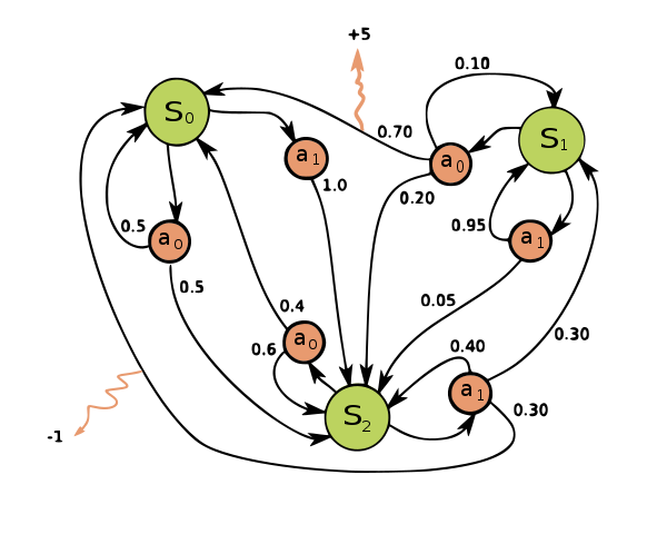
The objective of an MDP is to design an agent that produces the optimal policy, \(\pi^{\ast} \in \Pi\), that receives as high total cumulative rewards as possible in the shortest travel distance. Consider the following MDP.

Markov decision process from Wikimedia Commons
	$$ \begin{equation} \mathcal{S} = \{ s_{0} , s_{1} , s_{2} \} \qquad \mathcal{A} = \{ a_{0} , a_{1} \} \\ r ( s_{0} , a_{1} , s_{2} ) = -1 \qquad r ( s_{0} , a_{0} , s_{1} ) = +5 \end{equation} $$
	$$ \begin{align} \mathbf{P} ( a_{0} ) & = \begin{bmatrix} p ( s_{0} \vert s_{0} , a_{0} ) & p ( s_{1} \vert s_{0} , a_{0} ) & p ( s_{2} \vert s_{0} , a_{0} ) \\ p ( s_{0} \vert s_{1} , a_{0} ) & p ( s_{1} \vert s_{1} , a_{0} ) & p ( s_{2} \vert s_{1} , a_{0} ) \\ p ( s_{0} \vert s_{2} , a_{0} ) & p ( s_{1} \vert s_{2} , a_{0} ) & p ( s_{2} \vert s_{2} , a_{0} ) \\ \end{bmatrix} \\ & = \begin{bmatrix} 0.5 & 0.0 & 0.5 \\ 0.7 & 0.1 & 0.2 \\ 0.4 & 0.0 & 0.6 \\ \end{bmatrix} \\ \mathbf{P} ( a_{1} ) & = \begin{bmatrix} p ( s_{0} \vert s_{0} , a_{1} ) & p ( s_{1} \vert s_{0} , a_{1} ) & p ( s_{2} \vert s_{0} , a_{1} ) \\ p ( s_{0} \vert s_{1} , a_{1} ) & p ( s_{1} \vert s_{1} , a_{1} ) & p ( s_{2} \vert s_{1} , a_{1} ) \\ p ( s_{0} \vert s_{2} , a_{1} ) & p ( s_{1} \vert s_{2} , a_{1} ) & p ( s_{2} \vert s_{2} , a_{1} ) \\ \end{bmatrix} \\ & = \begin{bmatrix} 0.0 & 0.0 & 1.0 \\ 0.0 & 0.95 & 0.05 \\ 0.3 & 0.3 & 0.4 \\ \end{bmatrix} \end{align} $$

Since the objective is to acquire high rewards, the agent should move towards positive rewards and avoid negative rewards. Therefore, the optimal policy, \(\pi^{\ast} \in \Pi\) is:

\[\begin{equation} \pi^{\ast} ( a \vert s ) = \begin{bmatrix} \pi ( a_{0} \vert s_{0} ) & \pi ( a_{1} \vert s_{0} ) \\ \pi ( a_{0} \vert s_{1} ) & \pi ( a_{1} \vert s_{1} ) \\ \pi ( a_{0} \vert s_{2} ) & \pi ( a_{1} \vert s_{2} ) \\ \end{bmatrix} = \begin{bmatrix} 0.0 & 1.0 \\ 1.0 & 0.0 \\ 0.0 & 1.0 \\ \end{bmatrix} \end{equation}\]

A policy can be:

• Deterministic: The choice of action is non-probabilistic, so the next action is produced for a given state, or \(a = \pi ( a \vert s )\).
• Stochastic: The choice of action is probabilistic, so the next action is sampled from policy distribution, or \(a \sim \pi ( a \vert s ) \in \mathbb{R}^{m}\), where \(\sum_{a \in \mathcal{A}} \pi ( a \vert s ) = 1\).

Any type of policy can be used for any type of MDPs, i.e. a deterministic policy in a stochastic MDP or a stochastic MDP in a deterministic MDP.

Both have pros and cons. In the optimal world, where you can fully observe how the environment dynamics work, which is the above example, the optimal policy is deterministic, but in the real world, the stochastic policy is usually preferred because:

• Deterministic policy lacks diversity (exploration-exploitation dilemma).
• The agent does not fully observe states in many practical scenarios (partial observability).

A good example is an aliased gridworld from Stanford CS234 lecture.

Ergodicity

The ergodicity is a good property for an MDP to hold, but this is more complicated than an MC due to the presence of the actions and the policy. Consider that the agent is in an enemy is in front of me state with two available actions, attack and wait. When the agent executes attack, the agent may or may not defeat the enemy.

1. With \(p (\) an enemy is defeated \(\vert\) an enemy is in front of me, attack \()\), the agent reaches an enemy is defeated state.
2. With \(p (\) an enemy dodged attack \(\vert\) an enemy is in front of me, attack \()\), the agent reaches an enemy dodged attack state.

The agent might require to execute attack until it reaches an enemy is defeated state. However, if the agent executes wait, it will reach an enemy killed you state, or \(p (\) an enemy killed you \(\vert\) an enemy is in front of me, wait \() = 1\). If the agent dies, it can never return to an enemy is in front of me state again.

• If there is even a small chance of selecting wait, \(\pi (\) wait \(\vert\) an enemy is in front of me \() > 0\), an MDP has absorbing states or chains.
• If there is no chance of selecting wait, \(\pi (\) wait \(\vert\) an enemy is in front of me \() = 0\), an MDP has only positive recurrent states.

However, unlike an MC, having absorbing states or chains does not mean that the MDP is absorbing. More formally, define a state stationary distribution, stationary distribution or steady-state distribution, \(d ( s )\):

\[\begin{align} d ( s ) = & \lim_{t \rightarrow \infty} \Pr (S_{t} = s \vert s_{0} , \pi) \\ \equiv & \sum_{k=0}^{\infty} \Pr ( S_{0} = s_{0} \rightarrow S_{k} = s \vert k , \pi) = \sum_{k=0}^{\infty} \Pr (s_{0} \rightarrow s \vert k , \pi) \end{align}\]

Similar to an MC, it is the probability distribution over states that you will end up if you travel an MDP infinitely under \(\pi\).

• The first term signifies that for a given \(S_{0} = s_{0}\), the probability that the agent travels to \(s\) when \(t \rightarrow \infty\) following \(\pi\).
• The second term signifies the summation of the probability that the agent travels from \(S_{0} = s_{0}\) to \(s\) at \(k\) number of steps following \(\pi\) across \(k = 0\) to \(\infty\). This is often referred to as a state visitation probability.

\[\begin{align} \Pr (s \rightarrow s \vert 0 , \pi ) = & 1 \\ \Pr (s \rightarrow s' \vert 0 , \pi ) = & 0 \\ \Pr (s \rightarrow s' \vert 1 , \pi ) = & \sum_{a \in \mathcal{A}} \pi ( a \vert s ) p ( s' \vert s , a ) \\ \Pr (s \rightarrow s'' \vert k , \pi ) = & \sum_{s' \in \mathcal{S}} \Pr (s \rightarrow s' \vert n, \pi ) \cdot \Pr (s' \rightarrow s'' \vert k - n , \pi ) \end{align}\]

Furthermore, \(d\) can be represented recursively.

\[\begin{equation} d ( s' ) = \sum_{s \in \mathcal{S}} d ( s ) \sum_{a \in \mathcal{A}} \pi ( a \vert s ) p ( s' \vert s , a ) \end{equation}\]

Before getting into the ergodicity, there is one additional class of an MDP. An unichain MDP is an MDP that guarantees a unique stationary state distribution for every policy, but its visitation is not guaranteed for every state. This means that the unichain MDP has a unique stationary state distribution that contains \(d (s) = 0\) for some \(s\), therefore, not ergodic.

There seems to be no formal definition on the ergodicity in an MDP, but three different definitions I found from What is ergodicity in a Markov Decision Process (MDP)? are:

• There exists a policy \(\pi\) for a unique stationary distribution, \(d ( s )\), such that \(d ( s ) > 0\) from Moldovan.
• For every policy \(\pi\), a unique stationary distribution exists, \(d ( s )\), such that \(d ( s ) > 0\) from Puterman.
• For every policy \(\pi\), a unique stationary distribution exists, \(d ( s )\), such that \(d ( s ) \geq 0\) from Sutton.

Since the policy is usually learned, any of the definitions has a risk of falling into absorbing states. Most reinforcement learning takes the third definition, but it is not truly ergodic since a limiting distribution may reach zero for some \(\pi\).

• In many reinforcement learning problems, an ergodicity assumption breaks since closed irreducible sets are present in an MDP, i.e. the permanent damages to robots or the progress of the game stage. There is one interesting perspective on how the ergodicity deals with the safety of the agent, Safe Exploration in Markov Decision Processes by Moldovan.
• The research towards ergodicity in an MDP appears to be more related to operations research, so if you are interested, take a look at operations research.

Value Function

The optimal policy is to guide the agent towards states with the highest total cumulative rewards.

\[\begin{equation} \pi^{\ast} ( a \vert s ) = \arg \max_{\pi} \mathbb{E} [ \sum_{t = 0}^{\infty} r ( s_{t} ) ] \end{equation}\]

However, the agent must pursue the highest total cumulative rewards in the shortest travel distance. \(\sum_{t = 0}^{\infty} r ( s_{t} )\) weights the significance of the rewards in short distance and long distance equal. Then, the agent may potentially:

• Fall into an infinite loop, where it repetitively visits the same states with rewards.
• Aim for only large but distant rewards, where it ignores many small rewards in a short distance.

To comprehend the length of the travel distance into the optimal policy, we include a discount factor inside the optimization, often referred to as a return that is the total discounted cumulative rewards that the agent received throughout the trajectory, \(R_{t} = \sum_{k = 0}^{\infty} \gamma^{k} r ( s_{t + k + 1} )\).

\[\begin{equation} \pi^{\ast} ( a \vert s ) = \arg \max_{\pi} \mathbb{E} [ R_{t} ] = \arg \max_{\pi} \mathbb{E} [ \sum_{k = 0}^{\infty} \gamma^{k} r ( s_{t + k + 1} ) ] \end{equation}\]

Appropriately selecting \(\gamma \in [0,1]\) diminishes the effects of the long-distance rewards when computing the return.

• If \(\gamma = 0\), the agent only cares about rewards in a single step, or short-sighted, which may result in the agent not learning anything if the rewards are sparse.
• If \(\gamma = 1\), the agent cares about rewards of the infinite horizon, or long-sighted, which may fall into an infinite loop or care about high but far-to-reach rewards.

You can view short-sighted and long-sighted from the Stanford marshmallow experiment. A discount factor has a mathematical property that is bounded by \(\sum_{k = 0}^{\infty} \gamma^{k} = \frac{ 1 }{ 1 - \gamma }\). There are other ways to balance short- and long-sighted and they have different mathematic properties.

Additionally, \(d\) also includes a discount factor in its expression.

\[\begin{align} d ( s ) = & \lim_{t \rightarrow \infty} \gamma^{t} \Pr (S_{t} = s \vert s_{0} , \pi) \end{align}\]

To make the mathematical expression of the optimization more flexible for reinforcement learning algorithms, we use the expectation of a return, or a value function.

\[\begin{equation} v ( s ) = \mathbb{E} [ R_{t} \vert S = s ] \qquad q ( s , a ) = \mathbb{E} [ R_{t} \vert S = s , A = a ] \end{equation}\]

Where \(v\) is a state value function or state value, and \(q\) is a state-action value function or Q value. \(v\) quantifies how good a particular state is based on the expected return from the state following the policy while \(q\) deals with a state and action pair.

Thus, the optimal policy is expressed as:

\[\begin{align} \pi^{\ast} ( a \vert s ) = & \arg \max_{\pi} \mathbb{E} [ R_{t} ] \\ \equiv & \arg \max_{\pi} \mathbb{E} [ v ( s ) ] = \arg \max_{\pi} \sum_{s \in \mathcal{S}} d ( s ) v ( s ) \\ \equiv & \arg \max_{\pi} \mathbb{E} [ q ( s , a ) ] = \arg \max_{\pi} \sum_{s \in \mathcal{S}} d ( s ) \sum_{a \in \mathcal{A}} \pi ( a \vert s ) q ( s , a ) \end{align}\]

An average-reward continuous MDP formalizes the value functions differently. It represents the expected average reward without a discount factor.

\[\begin{equation} v ( s ) = \sum_{t = 1}^{\infty} \mathbb{E} \left[ r_{t} - R_{t} \vert S = s \right] \qquad q ( s , a ) = \sum_{t = 1}^{\infty} \mathbb{E} \left[ r_{t} - R_{t} \vert S = s , A = a \right] \end{equation}\]

Bellman Equation

In an MDP, the Bellman equation is a recursion of value functions. The fundamental idea is more abstract, where it deals with a necessary condition for optimality in dynamic programming, but here, I will just cover the simplest application of the Bellman equation in an MDP.

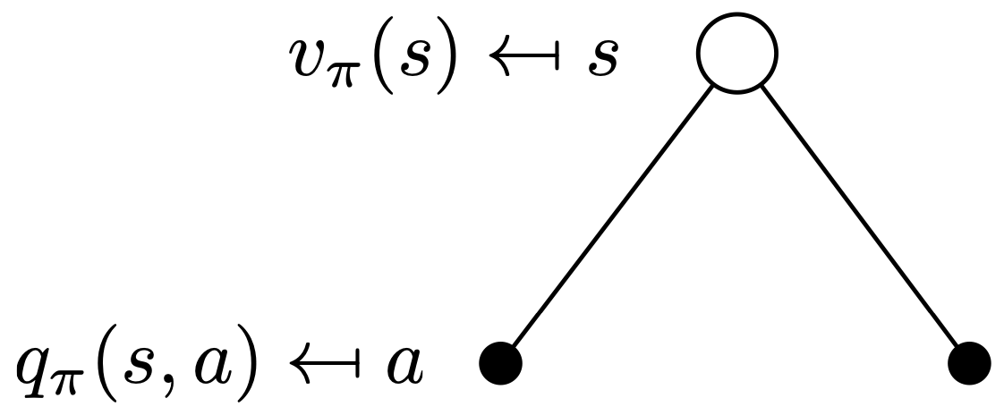
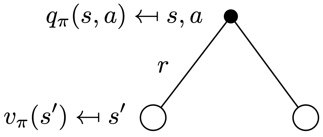
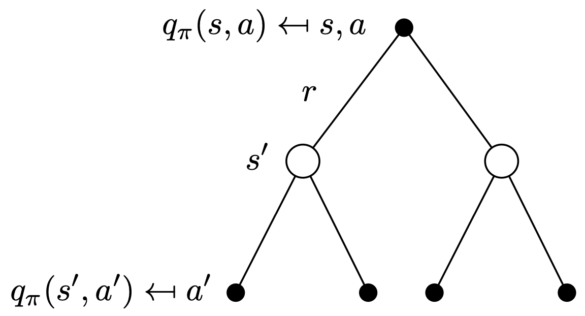
The Bellman expectation equation is a type of Bellman equations that decomposes the value function recursively into a reward and discounted future value function. Consider a white circle as a state and a black dot as an action:

Bellman expectation equation from David Silver's lecture

State value	Q value
$$ \begin{align} v (s) = \sum_{a \in A} \pi (a \vert s) q (s, a) \end{align} $$	$$ \begin{align} q (s, a) = \sum_{s' \in S} p (s' \vert s , a) \left( r ( s , a , s' ) + \gamma v (s') \right) \end{align} $$

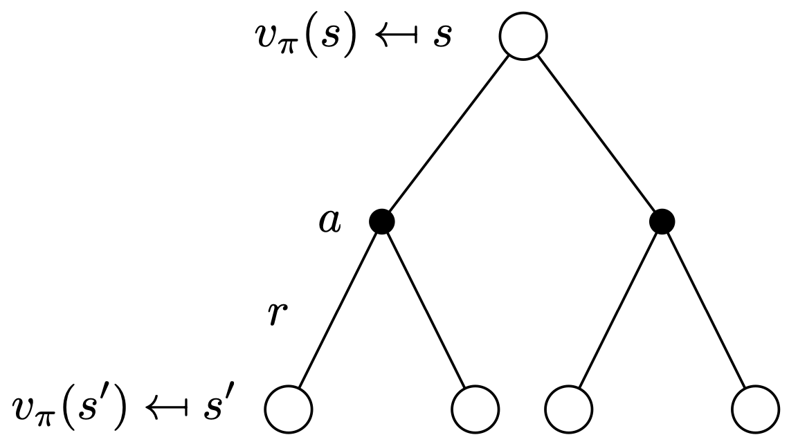
Two value functions can be combined to become recursive.

Bellman expectation equation 2 from David Silver's lecture

State value	Q value
$$ \begin{align} v (s) = \sum_{a \in A} \pi (a \vert s) \left( \sum_{s' \in S} p (s' \vert s , a) \left( r ( s , a , s' ) + \gamma v (s') \right) \right) \end{align} $$	$$ \begin{align} q (s, a) = \sum_{s' \in S} p (s' \vert s , a) \left( r ( s , a , s' ) + \gamma \sum_{a' \in A} \pi (a' \vert s') q (s', a') \right) \end{align} $$

The Bellman optimality equation is another Bellman equation, which is basically the Bellman expectation equation with the greedy policy.

\[\begin{equation} \pi^{\ast} ( a \vert s ) = \begin{cases} 1 & \arg \max_{a} q ( s , a ) \\ 0 & \text{otherwise} \end{cases} \end{equation}\]

The greedy policy is a type of deterministic policies, driven by only the maximum \(q ( s , a )\). Then, the two value functions can be formulated as:

\[\begin{equation} v^{\ast} (s) = \sum_{a \in A} \pi^{\ast} (a \vert s) q^{\ast} (s, a) = \max_{a} q^{\ast} (s, a) \\ q^{\ast} (s, a) = \sum_{s' \in S} p (s' \vert s , a) \left( r ( s , a , s' ) + \gamma v^{\ast} (s') \right) \end{equation}\]

Furthermore, recursively:

\[\begin{equation} v^{\ast} (s) = \max_a \left( \sum_{s' \in S} p (s' \vert s , a) ( r ( s , a , s' ) + \gamma v^{\ast} (s')) \right) \\ q^{\ast} (s, a) = \sum_{s' \in S} p (s' \vert s , a) \left( r ( s , a , s' ) + \gamma \max_{a'} q^{\ast} (s', a') \right) \end{equation}\]

Often notations vary:

• \(d^{\pi}\): The state stationary distribution following the policy, for instance, \(d^{\pi} ( s ) \neq d^{\pi'} ( s )\).
• \(v_{\pi}\): The state value following the policy, for instance, \(v_{\pi} ( s ) \neq v_{\pi'} ( s )\).
• \(R ( s_{t} , a_{t} )\): The return at \(s_{t}\) and \(a_{t}\), for instance, \(R_{t} = R ( s_{t} , a_{t} )\).
• \(\mathbb{E}_{ \tau \sim \pi }\): The expectation such that the trajectories are sampled following the policy, for instance, \(v_{\pi} (s) = \mathbb{E}_{ \tau \sim \pi } [ R_{t} \vert S = s ]\).
• \(\mathbb{E}_{ s \sim d^{\pi} , a \sim \pi }\): The expectation such that the state is sampled from the state stationary distribution and the action is from the policy, for instance, \(\mathbb{E}_{ \tau \sim \pi } [ R_{t} \vert S = s ] = \mathbb{E}_{ s \sim d^{\pi} , a \sim \pi } [ R_{t} \vert S = s ]\).
• The mathematical expressions of the Bellman expectation and optimality equations might be different from other articles or lectures. This is because a reward function takes different inputs, i.e. \(r ( s , a )\) or \(r ( s )\), but there is no practical difference.
• The exact same notations are applied to the Q value.

Extensions to Markov Decision Process

An MDP is a fully observable fixed environment with only a single player. There are a number of extended MDPs commonly used in reinforcement learning.

Partial Observability

A partially observable Markov decision process (POMDP) is an MDP with partial observability. Instead of observing states directly, the agent receives an observation, infers a state and executes an action. A POMDP can be seen as an HMM version of an MDP, a tuple of \(( \mathcal{S}, \mathcal{A}, \mathcal{P}, \mathcal{O}, \mathcal{P}_{o}, \mathcal{R}, \gamma )\), where \(\mathcal{O}\) is the observation space and \(\mathcal{P}_{o}\) is the conditional observation probability. \(\mathcal{P}_{o}\) also carries the Markov property.

\[\begin{align} \Pr ( O_{t} = o_{t} \vert S_{0:t} = s_{0:t} , A_{0:t-1} = a_{0:t-1} ) \equiv & p_{o} ( O_{t} = o_{t} \vert S_{t} = s_{t} , A_{t-1} = a_{t-1} ) \\ = & p_{o} ( o_{t} \vert s_{t} , a_{t} ) \end{align}\]

The conditional observation probability can be written as \(\mathcal{P}_{o} : \mathcal{S} \rightarrow \mathcal{O}\) or \(\mathcal{P}_{o} : \mathcal{S} \times \mathcal{A} \rightarrow \mathcal{O}\), but others share the same with MDP.

In the classic POMDP, a belief, \(b (s)\), is used to infer the state, which is a probability distribution over states. Then, the state can be inferred from:

\[\begin{equation} b'( s' ) = \eta \cdot p_{o} ( o' \vert s' , a ) \sum_{ s \in \mathcal{S} } p ( s' \vert s , a ) b ( s ) \end{equation}\]

Where \(\eta = \frac{1}{ \Pr ( o \vert b , a ) }\) is a normalizing constant with:

\[\begin{equation} \Pr ( o \vert b , a ) = \sum_{ s' \in \mathcal{S} } p_{o} ( o' \vert s' , a ) \sum_{ s \in \mathcal{S} } p ( s' \vert s , a ) b ( s ) \end{equation}\]

• \(\sum_{ s \in \mathcal{S} } p ( s' \vert s , a ) b ( s )\): For an action that we executed, we multiply the state probability in the belief to the state transition probability for the next state, then we sum all across every state. This will give us the probability that we will reach at \(s'\) for a given \(a\), or \(\Pr ( s' \vert a )\).
• \(p_{o} ( o' \vert s' , a ) \Pr ( s' \vert a )\): For an acquired observation \(o'\), we can multiply the conditional observation probability of \(o'\) for \(s'\) and \(a\) pair to \(\Pr ( s' \vert a )\) to get the unnormalized probability that we are in \(s'\) for a given \(o'\) and \(a\). This is the unnormalized belief.
• \(b( s )\): A probability distribution over states that determines where the agent would be at the current time step.

However, in deep reinforcement learning, instead, we often use a neural network as a function that maps from the observation space to the state space, \(f : \mathcal{O} \rightarrow \mathcal{S}\).

Other Environments

A more general setting to a POMDP is a decentralized POMDP (Dec-POMDP), where multiple agents are involved in decision making. It considers uncertainty in outcomes, sensors and communications. A Dec-POMDP is a 7-tuple \(( \mathcal{S}, \{ \mathcal{A}_{i} \}, \mathcal{P}, \{ \mathcal{O}_{i} \}, \mathcal{P}_{o}, \mathcal{R}, \gamma )\), where there are \(i\) number of agents, so \(i\) number of acquirable observations and executable actions. Hence, a POMDP is a special case of a Dec-POMDP with a single agent.

Further generalization on Dec-POMDP is a partially observable stochastic game (POSG). The agents in a POSG hold different rewards, \(( \mathcal{S}, \{ \mathcal{A}_{i} \}, \mathcal{P}, \{ \mathcal{O}_{i} \}, \mathcal{P}_{o}, \{ \mathcal{R}_{i} \}, \gamma )\), so they either compete or cooperate in pursuing their assigned rewards. The terminology is from a game theory, where a stochastic game, or Markov game, refers to a repeated game with probabilistic transitions played by one or more players while partially observable is equivalent to adding observations and emission probabilities to the stochastic game.

An MDP can also hold non-stationarity, referred to as a non-stationary MDP (NSMDP). It is simply a varying MDP over time or epoch, formally \(\mathcal{M}^{(i)} = ( \mathcal{S}^{(i)}, \mathcal{A}^{(i)}, \mathcal{P}^{(i)}, \mathcal{R}^{(i)}, \gamma^{(i)} )\), where there is \(i \in \mathbb{R}\). A special case of an NSMDP is used for multi-task reinforcement learning, meta reinforcement learning, and continual reinforcement learning, i.e. \(\mathcal{M}^{(i)} = ( \mathcal{S}, \mathcal{A}, \mathcal{P}, \mathcal{R}^{(i)}, \gamma )\) if the environment does not change. Note that this can also be applied to a POMDP, \(\mathcal{M}^{(i)} = ( \mathcal{S}^{(i)}, \mathcal{A}^{(i)}, \mathcal{P}^{(i)}, \mathcal{O}^{(i)}, \mathcal{P}_{o}^{(i)}, \mathcal{R}^{(i)}, \gamma^{(i)} )\).

If you are interested in further generalizations in an MDP, please read this blog.

Environments

Environments can be modelled with few properties.

• Environment can be:
  • Stochastic: Multiple states can be reached via an action for a given state, or there exist two or more states that have \(p ( s' \vert s , a ) \in (0, 1)\).
  • Deterministic: Only a single state can be reached via an action for a given state, or there exists a single state that has \(p ( s' \vert s , a ) = 1\).
• A state, action and time can be:
  • Discrete: State space, action space and time are countable, or there exists \(\mathcal{S} = \{ s_{i} \}_{i = 0}^{N}\), \(\mathcal{A} = \{ a_{i} \}_{i = 0}^{M}\), and \(\mathcal{T} = \{ t_{i} \}_{i = 0}^{K}\), where \(\sum_{s \in \mathcal{S}} \sum_{a \in \mathcal{A}} p (s' \vert s , a) = 1\) and \(\sum_{a \in \mathcal{A}} \pi (s \vert a) = 1\).
  • Continuous: State space, action space and time are measurable, or there exists \(\mathcal{S} = \mathbb{R}^{n}\), \(\mathcal{A} = \mathbb{R}^{m}\), and \(\mathcal{T} = \mathbb{R}\), where \(\int_{S} \int_{A} p (s' \vert s , a) \text{ d}a \text{ d}s = 1\) and \(\int_{A} \pi (s \vert a) \text{ d}a = 1\).

Note that discrete state space is interpreted as there exists \(N\) number of states while in continuous, an infinitely many (uncountable) number of states exist in \(n\) space.

Fully Observable Environments

There are two typical fully observable environments.

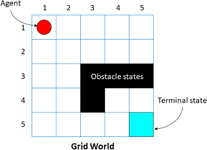
• Gridworld: Fully Observable Discrete Deterministic MDP
  • The agent ought to navigate (action) for a given location of the player (state) to solve the game (reward).

Gridworld from MathWorks

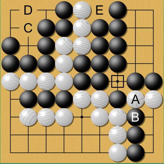
• Game Go in the two-player board game: Fully Observable Discrete Stochastic MDP
  • The agent ought to place a stone (action) for a given location of all the stones (state) to win the game (reward).
  • Many multi-player board games, including game Go and Chess, can be seen as either deterministic with multi-agent or stochastic with single-agent settings. For instance, the opponents can be seen as environment dynamics that induce stochasticity in the environment or other agents acting on the deterministic environment.
  • Many multi-player card games are often considered as discrete stochastic MDP with partial observability, a.k.a. a POMDP, or with no observation until the game finishes, a.k.a. an episodic MDP with a return at the end of the game.

Game Go from Wikimedia Commons

Partially Observable Environments

If the agent takes the state as an input, the environment becomes fully observable.

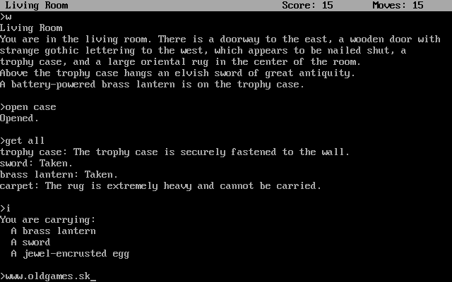
• Zork I in the text-based game: Discrete Stochastic POMDP
  • The agent ought to execute a textual command (action) for a given textual description of the world (observation) generated from the world graph (state) to solve puzzles in the game (reward).
  • Many text-based games are either deterministic or mild stochastic as they are designed to solve a set of specific tasks with limited causal relationships between entities. It is practically impossible to create infinitely many tasks with infinitely many causal relationships between entities.

Zork I from Old Games

• Space Invader in the arcade learning environment: Continuous state and Discrete action Stochastic POMDP
  • The agent ought to navigate or attack (action) for a given image of the world (observation) generated from the location of the player, enemies and items (state) to defeat the enemies (reward).
  • Similar to the game Go, every enemy can be seen as another fixed agent, but the environment is still stochastic since where the enemies and items appear is probabilistic.

Space invader from Wikipedia

• Robot Locomotion in the Open AI Gym: Continuous Deterministic POMDP.
  • The agent ought to move joints (action) for a given image of the world (observation) generated from the coordinates of the joints (state) to locomote as intended (reward).
  • If realistic factors are accounted, i.e. winds and terrains, it becomes stochastic.
  • Similar to the space invader, it can be a multi-agent setting if two or more robots are used to interact.

Robot locomotion from Wikimedia Commons

A time is discretized so that the agent can make a decision per time step. Note that by changing some factors, the environment can hold any property, i.e. gridworld with multi-agent setting or robot locomotion with a discrete action space \(\mathcal{A} = \{ 5 \text{m/s}, 10 \text{m/s} \}\). However, regardless of these properties, the policy and return are applied, so in practice:

• All the environments are formalized as a stochastic setting.
• In discrete MDP, the state is embedded using a high dimensional vector.
• In POMDP, the agent infers a high dimensional state, i.e. embedding or vector space, from observation using an encoder.

Summary

In this post, Markov models with a controllable system in a discrete-time setting are covered.

An MDP is a tuple of \(( \mathcal{S}, \mathcal{A}, \mathcal{P}, \mathcal{R}, \gamma )\), where a controllable system, or an agent, ought to 1) execute actions, \(a \in \mathcal{A}\); 2) following the policy, \(\pi \in \Pi\); 3) to navigate to the states, \(s \in \mathcal{S}\); 4) through state transition probabilities, \(p \in \mathcal{P}\); 5) that hold positive rewards, \(r \in \mathcal{R}\).

A policy, state transition probability and reward in an MDP follow the Markov property.

\[\begin{equation} \Pr ( A_{t} = a_{t} \vert S_{0:t} = s_{0:t} ) \equiv \pi ( A_{t} = a_{t} \vert S_{t} = s_{t} ) = \pi ( a_{t} \vert s_{t} , a_{t-1} ) \\ \Pr ( S_{t+1} = s_{t+1} \vert S_{0:t} = s_{0:t} , A_{0:t} = a_{0:t} ) \equiv p ( S_{t+1} = s_{t+1} \vert S_{t} = s_{t} , A_{t} = a_{t} ) = p ( s_{t+1} \vert s_{t} , a_{t} ) \\ r ( S_{0:t} = s_{0:t} , A_{0:t-1} = a_{0:t-1} ) \equiv r ( S_{t} = s_{t} , A_{t-1} = a_{t-1} , S_{t-1} = s_{t-1} ) = r ( s_{t} , a_{t-1} , s_{t-1} ) \end{equation}\]

A collection of states and actions that the agent travelled for a given maximum time, \(T\), is referred to as a trajectory, \(\{ S_{0} = s_{0} , A_{1} = a_{1} , \cdots A_{T-1} = a_{T-1} , S_{T} = s_{T} \}\).

• If \(T \rightarrow \infty\), an MDP is referred to as a continuous average-reward MDP, where the task may continue forever.
• If \(T < \infty\), an MDP is referred to as an episodic start-state MDP, where the task has a clear ending.

An MDP is all about the policy. A policy can be:

• Deterministic: The choice of action is non-probabilistic, so the next action is produced for a given state, or \(a = \pi ( a \vert s )\). Ideal for the optimal world, where environment dynamics are fully observed.
• Stochastic: The choice of action is probabilistic, so the next action is sampled from policy distribution, or \(a \sim \pi ( a \vert s ) \in \mathbb{R}^{m}\), where \(\sum_{a \in \mathcal{A}} \pi ( a \vert s ) = 1\). Ideal for the real world, where environment dynamics are not fully observed.

An MDP also has the concept of ergodicity, but the definition varies by literature.

• There exists a policy \(\pi\) for a unique stationary distribution, \(d ( s )\), such that \(d ( s ) > 0\) from Moldovan.
• For every policy \(\pi\), a unique stationary distribution exists, \(d ( s )\), such that \(d ( s ) > 0\) from Puterman.
• For every policy \(\pi\), a unique stationary distribution exists, \(d ( s )\), such that \(d ( s ) \geq 0\) from Sutton.
• Where:
  • A state stationary distribution, stationary distribution or steady-state distribution, \(d ( s )\):
  \[\begin{align} d ( s ) = & \lim_{t \rightarrow \infty} \Pr (S_{t} = s \vert s_{0} , \pi) \equiv \sum_{k=0}^{\infty} \Pr (s_{0} \rightarrow s \vert k , \pi) \\ = & \sum_{s' \in \mathcal{S}} d ( s' ) \sum_{a' \in \mathcal{A}} \pi ( a' \vert s' ) p ( s \vert s' , a' ) \end{align}\]
  • A state visitation probability, \(\Pr (s_{0} \rightarrow s \vert k , \pi )\):
  \[\begin{align} \Pr (s \rightarrow s' \vert 1 , \pi ) = \sum_{a \in \mathcal{A}} \pi ( a \vert s ) p ( s' \vert s , a ) \qquad \Pr (s \rightarrow s'' \vert k , \pi ) = \sum_{s' \in \mathcal{S}} \Pr (s \rightarrow s' \vert n, \pi ) \cdot \Pr (s' \rightarrow s'' \vert k - n , \pi ) \end{align}\]

A policy is all about the rewards.

1. The optimal policy is the policy that acquires the highest total cumulative rewards.

   \[\begin{equation} \pi^{\ast} ( a \vert s ) = \arg \max_{\pi} \mathbb{E} [ \sum_{t = 0}^{\infty} r ( s_{t} ) ] \end{equation}\]

2. The optimal policy is the policy that acquires the highest total cumulative rewards in the shortest travel distance. A return is to comprehend both the total cumulative rewards and the travel length into the optimal policy.

   \[\begin{equation} \pi^{\ast} ( a \vert s ) = \arg \max_{\pi} \mathbb{E} [ R_{t} ] = \arg \max_{\pi} \mathbb{E} [ \sum_{k = 0}^{\infty} \gamma^{k} r ( s_{t + k + 1} ) ] \end{equation}\]
   • If \(\gamma = 0\), the agent only cares about rewards in a single step, or short-sighted, which may result in the agent not learning anything if the rewards are sparse.
   • If \(\gamma = 1\), the agent cares about rewards of the infinite horizon, or long-sighted, which may fall into an infinite loop or care about high but far-to-reach rewards.

3. To make the mathematical expression of the optimization more flexible for reinforcement learning algorithms, we use the expectation of a return, or a value function. There are two types of value functions, a state value, \(v ( s ) = \mathbb{E} [ R_{t} \vert S = s ]\), and Q value, \(q ( s , a ) = \mathbb{E} [ R_{t} \vert S = s , A = a ]\). \(v\) quantifies how good a particular state is based on the expected return from the state following the policy while \(q\) deals with a state and action pair.

   \[\begin{align} \pi^{\ast} ( a \vert s ) \equiv & \arg \max_{\pi} \mathbb{E} [ v ( s ) ] = \arg \max_{\pi} \sum_{s \in \mathcal{S}} d ( s ) v ( s ) \\ \equiv & \arg \max_{\pi} \mathbb{E} [ q ( s , a ) ] = \arg \max_{\pi} \sum_{s \in \mathcal{S}} d ( s ) \sum_{a \in \mathcal{A}} \pi ( a \vert s ) q ( s , a ) \end{align}\]
   • The Bellman expectation equation decomposes the value function recursively into a reward and discounted future value function.
   \[\begin{align} v (s) = & \sum_{a \in A} \pi (a \vert s) q (s, a) = \sum_{a \in A} \pi (a \vert s) \left( \sum_{s' \in S} p (s' \vert s , a) \left( r ( s , a , s' ) + \gamma v (s') \right) \right) \\ q (s, a) = & \sum_{s' \in S} p (s' \vert s , a) \left( r ( s , a , s' ) + \gamma v (s') \right) = \sum_{s' \in S} p (s' \vert s , a) \left( r ( s , a , s' ) + \gamma \sum_{a' \in A} \pi (a' \vert s') q (s', a') \right) \end{align}\]
   • The Bellman optimality equation is the Bellman expectation equation with the greedy policy.
   \[\begin{align} v^{\ast} (s) = & \sum_{a \in A} \pi^{\ast} (a \vert s) q^{\ast} (s, a) = \max_{a} q^{\ast} (s, a) = \max_a \left( \sum_{s' \in S} p (s' \vert s , a) ( r ( s , a , s' ) + \gamma v^{\ast} (s')) \right) \\ q^{\ast} (s, a) = & \sum_{s' \in S} p (s' \vert s , a) \left( r ( s , a , s' ) + \gamma v^{\ast} (s') \right) = \sum_{s' \in S} p (s' \vert s , a) \left( r ( s , a , s' ) + \gamma \max_{a'} q^{\ast} (s', a') \right) \end{align}\]

Some MDP variants are:

• Partially observable Markov decision process (POMDP): A tuple of \(( \mathcal{S}, \mathcal{A}, \mathcal{P}, \mathcal{O}, \mathcal{P}_{o}, \mathcal{R}, \gamma )\)

  \[\begin{align} \Pr ( O_{t} = o_{t} \vert S_{0:t} = s_{0:t} , A_{0:t-1} = a_{0:t-1} , O_{0:t-1} = o_{0:t-1} ) \equiv p_{o} ( O_{t} = o_{t} \vert S_{t} = s_{t} , A_{t-1} = a_{t-1} ) = p_{o} ( o_{t} \vert s_{t} , a_{t} ) \end{align}\]
  • A belief is used to infer the state.
  \[\begin{equation} b'( s' ) = \eta p_{o} ( o' \vert s' , a ) \sum_{ s \in \mathcal{S} } p ( s' \vert s , a ) b ( s ) \quad \text{where, } \eta = \frac{1}{ \Pr ( o \vert b , a ) } \end{equation}\] \[\begin{equation} \Pr ( o \vert b , a ) = \sum_{ s' \in \mathcal{S} } p_{o} ( o' \vert s' , a ) \sum_{ s \in \mathcal{S} } p ( s' \vert s , a ) b ( s ) \end{equation}\]
• Decentralized POMDP (Dec-POMDP): A tuple of \(( \mathcal{S}, \{ \mathcal{A}_{i} \}, \mathcal{P}, \{ \mathcal{O}_{i} \}, \mathcal{P}_{o}, \mathcal{R}, \gamma )\)
• Partially observable stochastic game (POSG): A tuple of \(( \mathcal{S}, \{ \mathcal{A}_{i} \}, \mathcal{P}, \{ \mathcal{O}_{i} \}, \mathcal{P}_{o}, \{ \mathcal{R}_{i} \}, \gamma )\)
• Non-stationary MDP (NSMDP): A tuple of \(\mathcal{M}^{(i)} = ( \mathcal{S}^{(i)}, \mathcal{A}^{(i)}, \mathcal{P}^{(i)}, \mathcal{R}^{(i)}, \gamma^{(i)} )\)

Reference

• Lecture 1 and 2 of David Silver’s lecture
• Chapter 3 in Reinforcement Learning: An Introduction

Other helpful resources are:

• MDP Cheatsheet Reference from John Schulman