Value-based Reinforcement Learning
Prerequisites
Machine intelligence is the last invention that humanity will ever need to make.
Nick Bostrom
If the universe is constructed with patterns and humans can interpret this, then so may machines. If machines become intelligent over humans, humans need not apply.
Machine learning is the study of algorithms that involve training a computer to learn patterns and relationships in data without being explicitly programmed. It can be divided into three types:
- Supervised Learning: The algorithm, or model, is trained on labeled data, where the goal is to map each input to the correct output.
- Unsupervised Learning: The algorithm, or model, is trained on unlabeled data, where the goal is to identify patterns or structure in the data without being told what to look for.
- Reinforcement Learning: The algorithm, or agent, is trained on the interactive worlds, where the goal is to learn a policy that maximizes rewards and minimize penalties.
The problems in ML can be largely divided by four types:
- Computer Vision: The problems require machines to interpret and understand visual data, i.e. images and videos. They includes image classification, object localization, video analysis, image captioning and visual question answering.
- Natural Language Processing: The problems require machines to interpret and understand human language, i.e. words and documents. They includes text classification, translation, summarization, speech analysis, question answering and dialogue system.
- Graph Analysis: The problems require machines to interpret and understand graph data, i.e. nodes and edges in graphs. They includes graph classification, link prediction, knowledge graph, social network analysis, recommendation system, combinatorial optimization and path finding.
- Decision Making: The problems require machines to interact with the world and choose an appropriate action based on data and objectives. They include game playing, autonomous vehicles and robotics.
Reinforcement learning is a subfield of machine learning, popular in decision making problems. The algorithms are generally grouped by:
| Value-based | Policy-based | |||
| Model-based | Model-free | |||
| Classic |
Policy Iteration,
Value Iteration |
Monte Carlo,
SARSA,
Q Learning |
Policy Gradient , Deterministic Policy Gradient | |
| Deep |
Deep Q Network, Double Deep Q Network,
Duel Deep Q Network, Rainbow |
Vanilla Policy Gradient, Natural Policy Gradient,
Trust Region Policy Optimization, Proximal Policy Optimization |
||
| Classic | Actor Critic | |||
| Deep |
Deep Deterministic Policy Gradient, Twin Delayed Deep Deterministic Policy Gradient,
Soft Q Learning, Soft Actor Critic |
|||
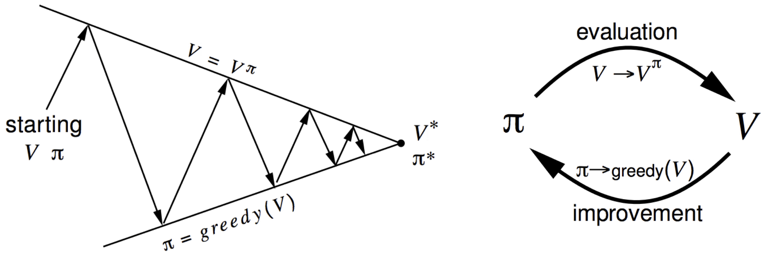
Value-based reinforcement learning (RL) is one of two fundamental classes of RL algorithms. It implicitly constructs the policy based on estimated value functions, so its objective is to correctly estimate value functions. The procedure is divided into two steps.
- Policy evaluation: A process of evaluating the policy by obtaining the Bellman equation.
- Policy improvement: A process of obtaining the improved policy based on the Bellman equation.
This post aims to provide a tutorial on value-based RL algorithms.
Policy Evaluation
The policy evaluation is a process of evaluating the policy by obtaining the Bellman equation. There are mainly three methods in the policy evaluation.
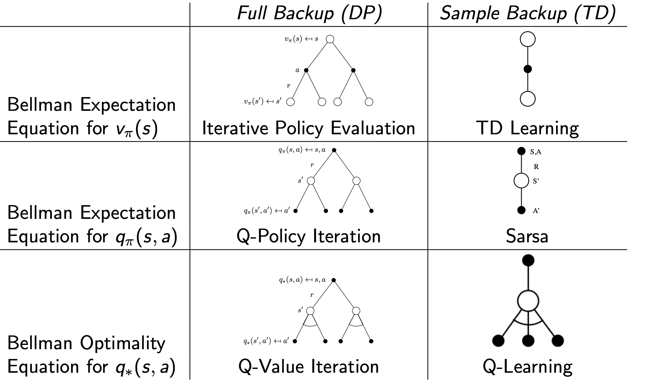
| Dynamic Programming | Temporal Difference | Monte Carlo |
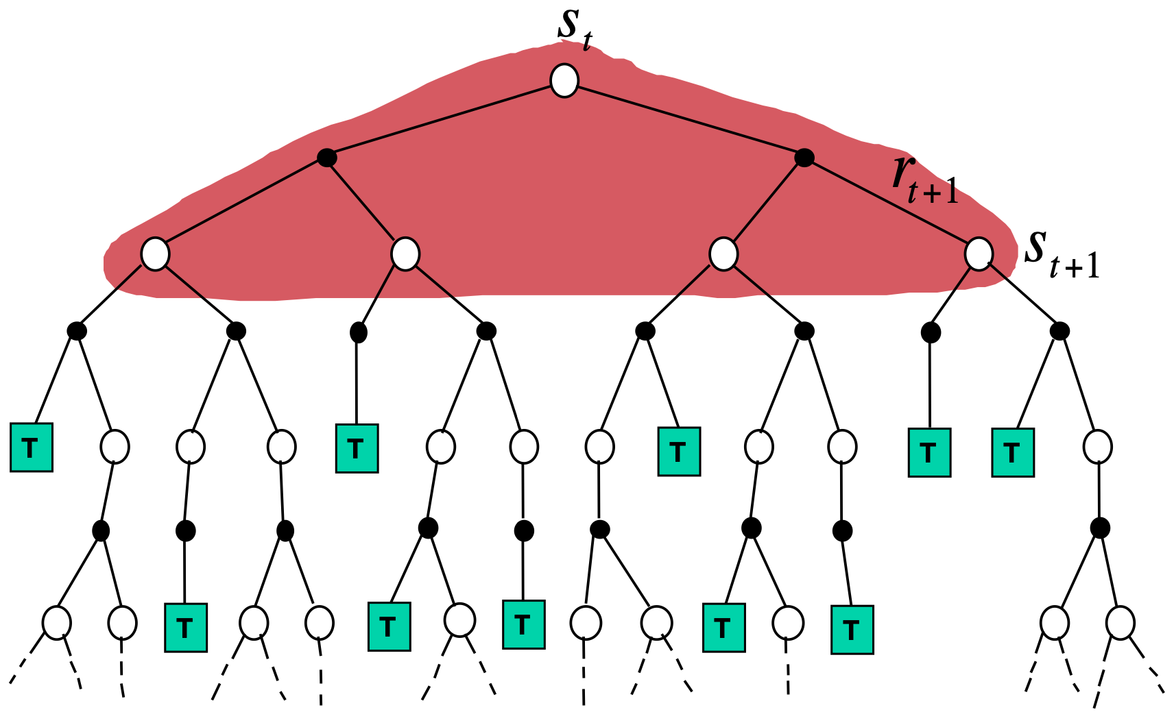
|
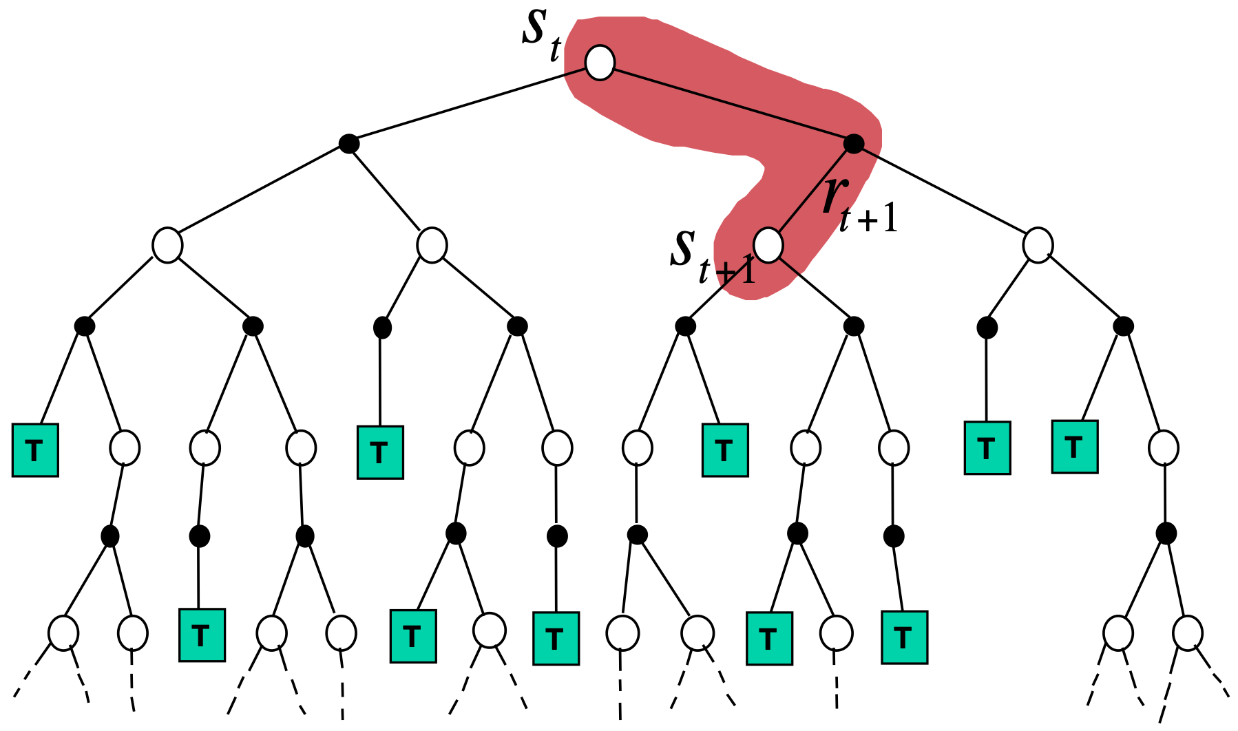
|
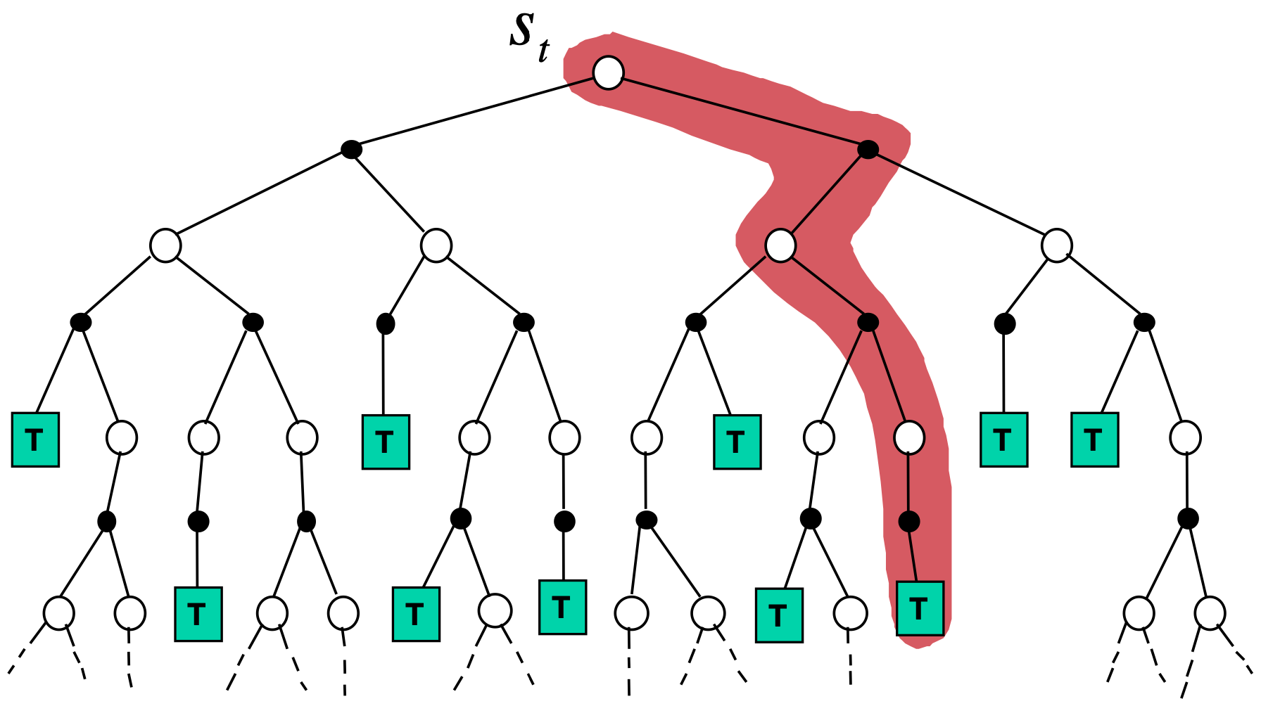
|
Where the update for the value functions is:
\[\begin{align} \text{DP: } & v_{\pi}^{(i+1)} ( s ) \leftarrow \sum_{a \in A} \pi (a \vert s) \left( \sum_{s' \in S} p (s' \vert s , a) \left( r' + \gamma \cdot v_{\pi}^{(i)} (s') \right) \right) \\ \text{TD: } & v_{\pi}^{(i+1)} ( s_{t} ) \leftarrow v_{\pi}^{(i)} ( s_{t} ) + \alpha \left( \left( r_{t+1} + \gamma v_{\pi}^{(i)} ( s_{t+1} ) \right) - v_{\pi}^{(i)} ( s_{t} ) \right) \\ \text{MC: } & v_{\pi}^{(i+1)} ( s_{t} ) \leftarrow v_{\pi}^{(i)} ( s_{t} ) + \alpha \left( \left( \sum_{k = 0}^{\infty} \gamma^{k} r_{t + k + 1} \right) - v_{\pi}^{(i)} ( s_{t} ) \right) \end{align}\]Where \(s \equiv s_{t}\) and \(s' \equiv s_{t+1}\). The notation \(s\) and \(s'\) signify the state and the neighbouring state while \(s_{t}\) and \(s_{t+1}\) signify the current state and the next state for a given trajectory, \(\tau = ( S_{0} = s_{0} , A_{0} = a_{0} , \cdots A_{T-1} = a_{T-1} , S_{T} = s_{T} )\).
Dynamic programming (DP) is both a mathematical optimization method and a computer programming method. It is a general idea of expressing a complex problem into simpler sub-problems, but in this post, I will focus on reinforcement learning (RL), in particular solving a Markov decision process (MDP). Note that this method is developed by Richard Bellman, which the Bellman equation is named after. DP simply iterates through all the states and actions to recursively update the value functions with full access to the environment dynamics of the MDP.
In practice, DP is not preferred as most of the environments are either 1) unknown MDPs, i.e. how the opponent will play the game Go is unknown, or 2) known but intractably large MDPs, i.e. the game Go has \(\vert \mathcal{S} \vert \approx 10^{170}\) and \(\vert \mathcal{A} \vert \approx 10^{360}\). To handle this, we often use sampling methods for the policy evaluation, which are divided into temporal difference (TD) or Monte-Carlo (MC). They do not require to access the environment dynamics, but instead, for a given \(\tau\), the states and actions are sampled for value function updates.
Comparison
Policy evaluation methods can be compared with respect to 1) sampling and 2) bootstrapping.
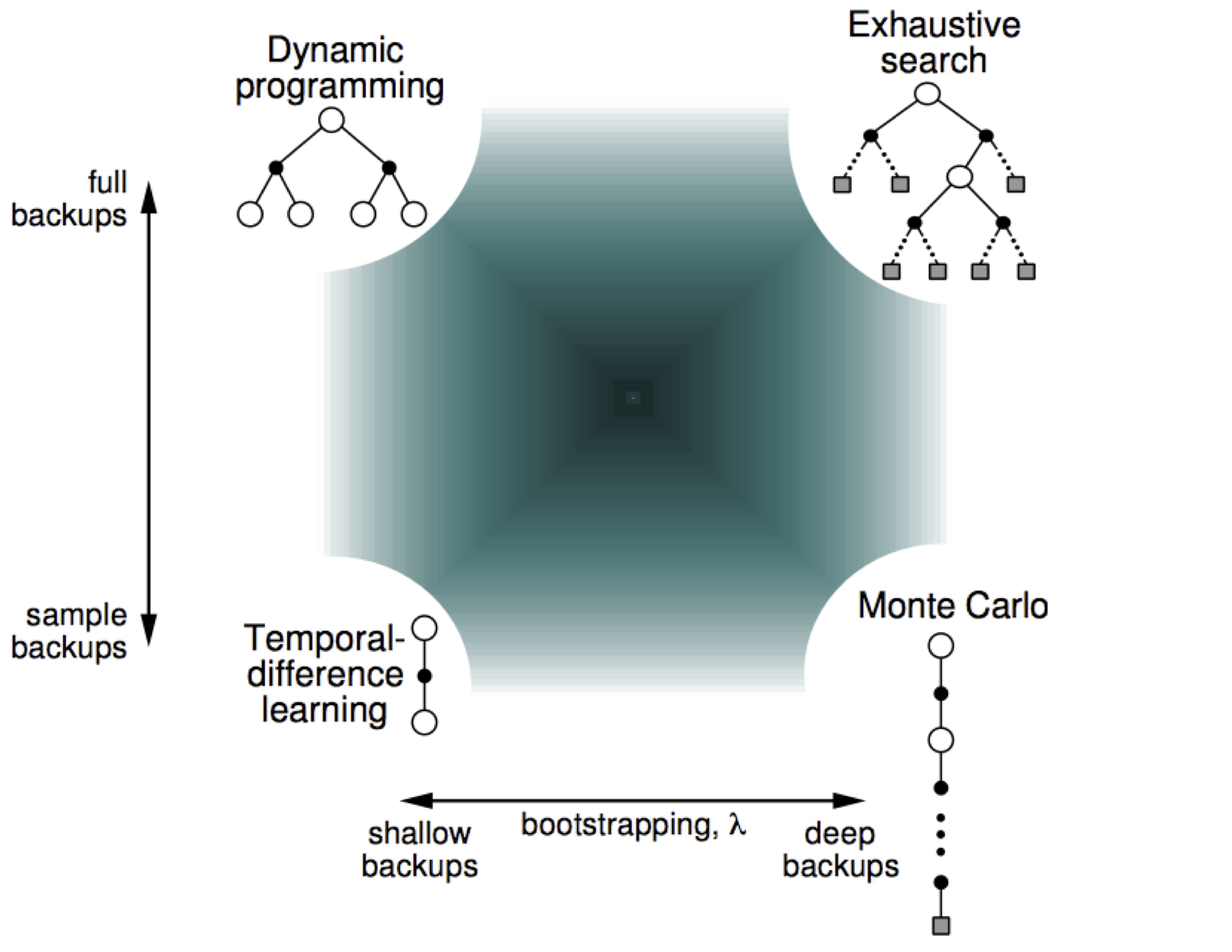
- Full backups account for every possible action to compute the Bellman equations while sample backups account for only sampled actions.
- Deep backups account for the entire trajectory to compute the Bellman equations while shallow backups account for only a single time step ahead.
While the term full backups and sample backups are used to describe the update method of the value functions, algorithms that utilize these techniques are referred differently:
- Model-based: The optimal policy is obtained using the environment dynamics, such as \(p ( s' \vert s , a )\).
- DP is known as model-based while the heuristic search can be model-based or model-free.
- Model-based algorithms include those models that do not access the environment dynamics, but learn and predict the environment dynamics. Thus, generally, any model-free algorithm with additional world predicting algorithms that help the update is considered model-based.
- Model-free: The optimal policy is obtained using sampled trajectories \(\tau\).
- Both TD and MC are considered model-free since they do not access nor predict environment dynamics.
- Majority of algorithms used in RL are model-free, but as mentioned, if additional world predicting algorithms are employed to help the update, they are classified as model-based.
The standard RL usually refers to model-free RL. TD and MC can further be generalized as:
\[\begin{equation} v_{\pi}^{(i+1)} ( s_{t} ) \leftarrow v_{\pi}^{(i)} ( s_{t} ) + \alpha \delta \quad \delta = \hat{v}_{\pi}^{(i)} ( s_{t} ) - v_{\pi}^{(i)} ( s_{t} ) \\ \hat{v}_{\pi}^{(i)} ( s_{t} ) = \begin{cases} r_{t+1} + \gamma v_{\pi}^{(i)} ( s_{t+1} ) & \text{for TD} \\ R_{t} = \sum_{k = 0}^{\infty} \gamma^{k} r_{t+k+1} & \text{for MC} \\ \end{cases} \end{equation}\]Where:
- \(\hat{v}_{\pi}^{(i)}\) is the estimated target value and \(v_{\pi}^{(i)}\) is the value.
- \(\delta\) is the difference between \(\hat{v}_{\pi}^{(i)}\) and \(v_{\pi}^{(i)}\), where \(\delta \rightarrow 0\) as \(i \rightarrow \infty\).
- Higher \(\alpha\) results in faster convergence, but may induce oscillations during learning.
- Lower \(\alpha\) results in slow convergence that may potentially result in falling into the local optima.
- The difference between TD and MC is how \(\hat{v}_{\pi}^{(i)}\) is constructed.
The idea of TD and MC is sampling techniques in the policy evaluation, where the update is done using trajectories that the agent travelled with the initial state distribution, \(p_{0}\), instead of accessing the state transition probabilities. While the policy evaluation differs, the policy improvement in TD and MC follows the greedy policy, the same as DP.
Bias and Variance
Model-free algorithms suffer from bias and variance problems since they use a sampling technique to update the value functions.
-
MC has no bias: Since \(v_{\pi} ( s_{t} ) = \mathbb{E}_{ \tau \sim \pi } \left[ R_{t} \vert s_{t} \right]\):
\[\begin{equation} \mathbb{E}_{ \tau \sim \pi } \left[ \hat{v}_{\pi}^{(i)} ( s_{t} ) \right] = \mathbb{E}_{ \tau \sim \pi } \left[ R_{t} \vert s_{t} \right] \equiv v_{\pi} ( s_{t} ) \end{equation}\] -
TD has bias: Since \(\hat{v}_{\pi}^{(i)} ( s_{t} ) = r_{t+1} + \gamma v_{\pi}^{(i)} ( s_{t+1} )\), \(\hat{v}_{\pi}^{(i)} ( s_{t} )\) follows \(v_{\pi}^{(i)} ( s_{t+1} )\), where \(v_{\pi}^{(i)} ( s_{t+1} )\) is an incorrect estimate. Thus, the initialization of the value functions causes bias in TD.
\[\require{color} \begin{align} v_{\pi}^{(i+1)} ( s_{t} ) & \leftarrow v_{\pi}^{(i)} ( s_{t} ) + \alpha \left( \hat{v}_{\pi}^{(i)} ( s_{t} ) - v_{\pi}^{(i)} ( s_{t} ) \right) \quad \hat{v}_{\pi}^{(i)} ( s_{t} ) = r_{t+1} + \gamma v_{\pi}^{(i)} ( s_{t+1} ) \\ & = \textcolor{red}{ v_{\pi}^{(i)} ( s_{t} ) + \alpha \left( \left( r_{t+1} + \gamma v_{\pi}^{(i)} ( s_{t+1} ) \right) - v_{\pi}^{(i)} ( s_{t} ) \right) } \\ & = \textcolor{blue}{ ( 1 - \alpha ) \cdot v_{\pi}^{(i)} ( s_{t} ) + \alpha \left( r_{t+1} + \gamma v_{\pi}^{(i)} ( s_{t+1} ) \right) } \\ & = ( 1 - \alpha ) \cdot \left( \textcolor{red}{ v_{\pi}^{(i-1)} ( s_{t} ) + \alpha \left( \left( r_{t+1} + \gamma v_{\pi}^{(i-1)} ( s_{t+1} ) \right) - v_{\pi}^{(i-1)} ( s_{t} ) \right) } \right) + \alpha \left( r_{t+1} + \gamma v_{\pi}^{(i)} ( s_{t+1} ) \right) \\ & = ( 1 - \alpha ) \cdot \left( \textcolor{blue}{ ( 1 - \alpha ) \cdot v_{\pi}^{(i-1)} ( s_{t} ) + \alpha \left( r_{t+1} + \gamma v_{\pi}^{(i-1)} ( s_{t+1} ) \right) } \right) + \alpha \left( r_{t+1} + \gamma v_{\pi}^{(i)} ( s_{t+1} ) \right) \\ & = ( 1 - \alpha )^{2} \cdot v_{\pi}^{(i-1)} ( s_{t} ) + \alpha ( 1 - \alpha )^{1} \left( r_{t+1} + \gamma v_{\pi}^{(i-1)} ( s_{t+1} ) \right) + \alpha ( 1 - \alpha )^{0} \left( r_{t+1} + \gamma v_{\pi}^{(i-0)} ( s_{t+1} ) \right) \\ & \; \vdots \\ & = ( 1 - \alpha )^{i} \cdot v_{\pi}^{(0)} ( s_{t} ) + \sum_{j = 0}^{i} \alpha ( 1 - \alpha )^{j} \left( r_{t+1} + \gamma v_{\pi}^{(i-j)} ( s_{t+1} ) \right) \end{align}\]- If \(i \rightarrow \infty\), then \(( 1 - \alpha )^{i} \cdot v_{\pi}^{(0)} ( s_{t} ) \rightarrow 0\). However, the second term still includes the value functions of the early time steps, i.e. \(\alpha ( 1 - \alpha )^{i-1} \left( r_{t+1} + \gamma v_{\pi}^{(1)} ( s_{t+1} ) \right)\). Thus, the bias decreases over time, but will not be removed. This is based on Why is temporal difference learning biased in reinforcement learning?.
-
MC has high variance: \(R_{t}\) at small \(t\) change drastically if \(a_{t}\) at small \(t\) change. Intuitively, in complex environments, there are infinitely many trajectories, but most of them are useless, so \(G_{0}\) for most trajectories will be zero or very small while there are some trajectories that produce relatively high \(G_{0}\).
\[\require{color} \begin{align} \text{Var} \left[ R_{t} \right] & = \text{Var} \left[ \sum_{k = 0}^{\infty} \gamma^{k} r_{t+k+1} \right] \\ & = \sum_{k = 0}^{\infty} (\gamma^{k})^{2} \text{Var} \left[ r_{t+k+1} \right] + \sum_{i \neq j} \gamma^{i} \cdot \gamma^{j} \cdot \text{Cov} \left[ r_{t+i+1}, r_{t+j+1} \right] \quad \text{Cov} \left[ r_{t+i+1}, r_{t+j+1} \right] = 0 \\ & = \sum_{k = 0}^{\infty} (\gamma^{k})^{2} \text{Var} \left[ r_{t+k+1} \right] + \sum_{i \neq j} \gamma^{i} \cdot \gamma^{j} \cdot 0 \\ & = \sum_{k = 0}^{\infty} (\gamma^{k})^{2} \text{Var} \left[ r_{t+k+1} \right] \\ & < \sum_{k = 0}^{\infty} \gamma^{k} \text{Var} \left[ r_{t+k+1} \right] \quad \text{where, } \gamma \in (0, 1) \end{align}\]- Note that \(\text{Cov} \left[ r_{t+i+1}, r_{t+j+1} \right] = 0\) is not really true since rewards in different time steps are correlated, but this is to provide a simple intuitive derivation. This is based on How does Monte Carlo have high variance?.
-
TD has low variance: This term ‘low’ is relative to MC. When computing \(\hat{v}_{\pi}^{(i)} ( s_{t} ) = r_{t+1} + \gamma v_{\pi}^{(i)} ( s_{t+1} )\), we do not account variance for rewards in the later time steps, and thus, the variance is \(\text{Var} \left[ r_{t+1} \right]\), which is smaller than \(\sum_{k = 0}^{\infty} \gamma^{k} \text{Var} \left[ r_{t+k+1} \right]\).
Thus, TD is known to have high bias and low variance, while MC is known to have low bias and high variance.
\(n\)-Step Bootstrapping
In RL, the bootstrapping is a process of computing \(\hat{v}_{\pi}^{(i)} ( s_{t} )\) based on \(v_{\pi}^{(i)} ( s_{t+1} )\). Instead of thoroughly relying on either TD or MC, we can use the \(n\)-step bootstrapping to balance bias and variance.
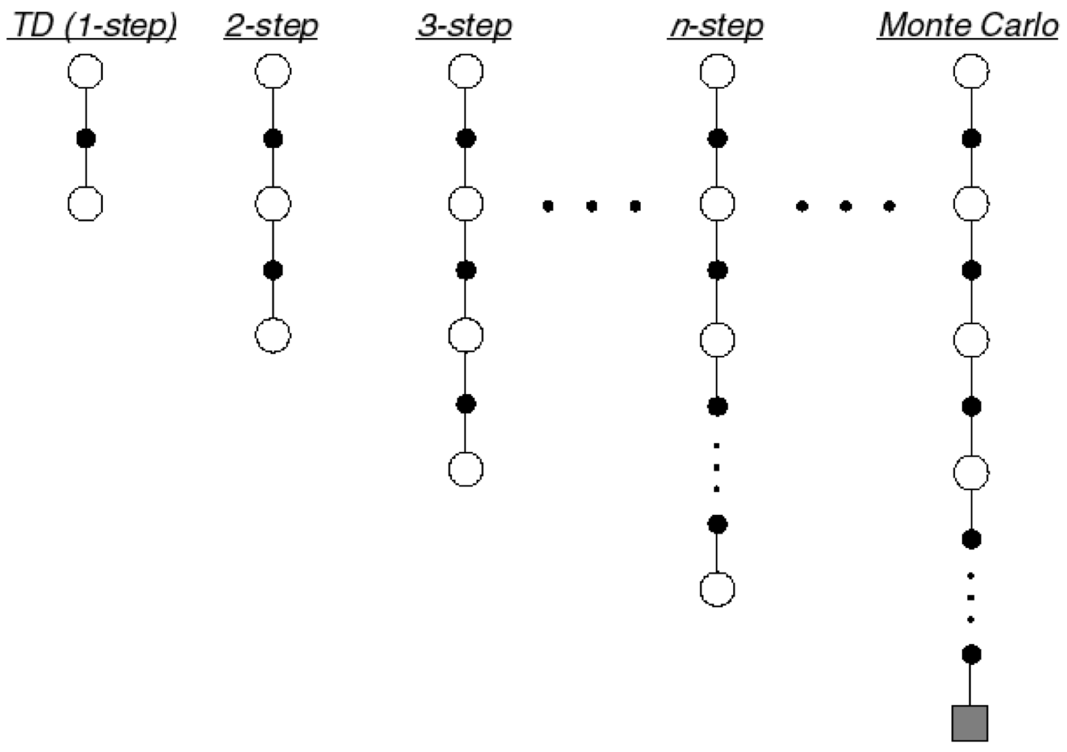
Where the update for the value functions is done according to:
\[\require{color} \begin{equation} \hat{v}_{\pi}^{(i)} ( s_{t} ) = R_{t}^{( \textcolor{red}{n} )} = \sum_{\textcolor{blue}{k} = 0}^{\textcolor{red}{n} - 1} \gamma^{\textcolor{blue}{k}} r_{t + \textcolor{blue}{k} + 1} + \gamma^{ \textcolor{red}{n} } v_{\pi}^{(i)} ( s_{t + \textcolor{red}{n}} ) \end{equation}\]The \(n\)-step bootstrapping with \(n = 1\) is the standard TD approach and \(n = \infty\) is equivalent to MC. Due to how it can balance bias and variance, the \(n\)-step bootstrapping with reasonable \(n\) is more preferred than MC.
Dynamic Programming
Since DP can provide nice intuition, I will go through some common algorithms in DP. There are two classes of value-based RL algorithms.
- Policy iteration: The policy evaluation with the Bellman expectation equation and the policy improvement.
- Value iteration: The policy evaluation with the Bellman optimality equation, which encapsulates the policy improvement with the greedy policy.
Policy Iteration
The policy iteration is to find the optimal policy with the Bellman expectation equation. There exist two policy iteration algorithms based on the type of value functions used in the policy evaluation.
- Generalized policy iteration, or V-policy iteration or iterative policy evaluation: The state value is used as a value function.
- Q-policy iteration: The Q value is used as a value function.
While the policy evaluation differs, the policy improvement usually uses the greedy policy.
\[\begin{equation} \pi_{\text{greedy}} ( a \vert s ) = \begin{cases} 1 & \arg \max_{a} q_{\pi} ( s , a ) \\ 0 & \text{otherwise} \end{cases} \end{equation}\]Where \(\pi_{\text{greedy}}\) is the most common example of the deterministic policy. Note that there are other ways to construct the policy in the policy improvement, i.e. the softmax policy, \(\pi_{\text{softmax}} ( a \vert s ) = \frac{ e^{ q_{\pi} ( s , a ) } }{ \sum_{a' \in \mathcal{A}} e^{ q_{\pi} ( s , a' ) } }\), for the stochastic policy.
The procedure of the generalized policy iteration follows:
- Policy evaluation: Obtain \(v_{\pi}^{(k)} ( s )\) for a given \(\pi^{(i)} ( a \vert s )\), where \(k\) is any reasonable number. Then, obtain \(q_{\pi}^{(i)} (s, a) = \sum_{s' \in S} p (s' \vert s , a) \left( r ( s , a , s' ) + \gamma v_{\pi}^{(k)} (s') \right)\) for the policy improvement.
- Policy improvement: Set \(\pi^{(i+1)} ( a \vert s )\) as the greedy policy for a given \(q_{\pi}^{(i)} (s, a)\).
- Policy iteration: Repeat the policy evaluation and the policy improvement to obtain \(\pi^{(\infty)} ( a \vert s ) \equiv \pi^{\ast} ( a \vert s )\).
Thus, this process is:
\[\begin{equation} \pi^{(0)} ( a \vert s ) \rightarrow v_{\pi}^{(0 \rightarrow k)} ( s ) \rightarrow q_{\pi}^{(1)} (s, a) \rightarrow \pi^{(1)} ( a \vert s ) \rightarrow \cdots \rightarrow \pi^{(\infty)} ( a \vert s ) \end{equation}\]The generalized policy iteration requires computing the Q value additionally to obtain the policy.
Example
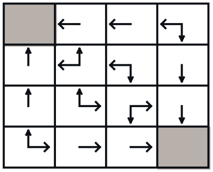
Consider a 4-by-4 deterministic gridworld problem with action set, \(\mathcal{A} = \{ N, S, E, W \}\).
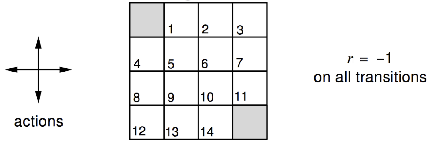
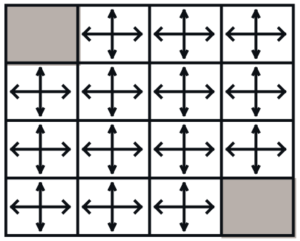
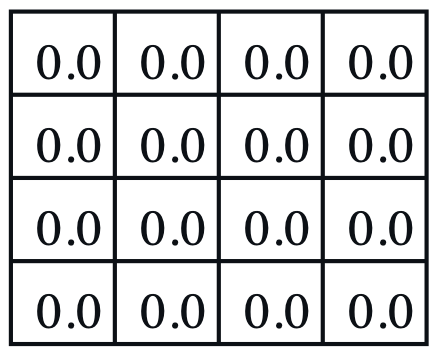
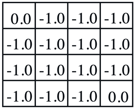
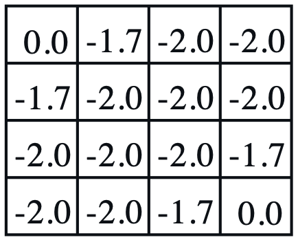
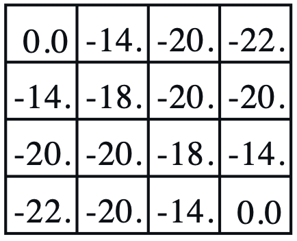
The grey regions are the terminal states and a reward is held in every state transition, \(r_{t+1} = r ( s_{t} , a_{t} , s_{t+1} ) = -1\). Let the initial policy be a uniform distribution over action, \(\pi^{(0)} ( a \vert s ) = \mathcal{U} ( \mathcal{A} )\), then, the value functions are computed by applying the Bellman expectation equation repetitively.
| $$ \pi^{(0)} ( a \vert s ) $$ | $$ v_{\pi}^{(0)} ( s ) $$ | $$ v_{\pi}^{(1)} ( s ) $$ | $$ v_{\pi}^{(2)} ( s ) $$ | $$ v_{\pi}^{(\infty)} ( s ) $$ | $$ \pi^{(1)} ( a \vert s ) $$ |
|
|
|
|
|
|
- Policy evaluation: For a given \(\pi^{(0)} ( a \vert s )\), iterate value functions until it converges, \(v_{\pi}^{(0)} ( s ) \rightarrow v_{\pi}^{(\infty)} ( s )\),
- The grey regions have \(v_{\pi}^{(\infty)} ( s ) = 0\) since it is the terminal state, no action is available.
- Policy improvement: Update the policy with actions from low to high value functions, \(\pi^{(0)} ( a \vert s ) \rightarrow \pi^{(1)} ( a \vert s )\). For instance, define \(\pi ( a \vert s ) = \begin{bmatrix} p_{N} & p_{S} & p_{E} & p_{W} \end{bmatrix}^{\intercal}\): \(\begin{equation} \pi^{(0)} ( a \vert s = 1 ) = \begin{bmatrix} \frac{1}{4} & \frac{1}{4} & \frac{1}{4} & \frac{1}{4} \end{bmatrix}^{\intercal} \quad \rightarrow \quad \pi^{(1)} ( a \vert s = 1 ) = \begin{bmatrix} 0 & 0 & 0 & 1 \end{bmatrix}^{\intercal} \\ \pi^{(0)} ( a \vert s = 2 ) = \begin{bmatrix} \frac{1}{4} & \frac{1}{4} & \frac{1}{4} & \frac{1}{4} \end{bmatrix}^{\intercal} \quad \rightarrow \quad \pi^{(1)} ( a \vert s = 2 ) = \begin{bmatrix} 0 & 0 & 0 & 1 \end{bmatrix}^{\intercal} \\ \pi^{(0)} ( a \vert s = 3 ) = \begin{bmatrix} \frac{1}{4} & \frac{1}{4} & \frac{1}{4} & \frac{1}{4} \end{bmatrix}^{\intercal} \quad \rightarrow \quad \pi^{(1)} ( a \vert s = 3 ) = \begin{bmatrix} 0 & \frac{1}{2} & 0 & \frac{1}{2} \end{bmatrix}^{\intercal} \end{equation}\)
In this example, \(k \rightarrow \infty\). In theory, under \(\pi^{(0)} ( a \vert s ) = \mathcal{U} ( \mathcal{A} )\), a single policy improvement with \(v_{\pi}^{(\infty)} ( s )\) is required for the optimal policy, \(\pi^{(1)} ( a \vert s ) \equiv \pi^{(\ast)} ( a \vert s )\). However, in practice, iterating through the policy evaluation and the policy improvement is more efficient. Thus, the generalized policy iteration usually switches between the policy evaluation and the policy improvement with a reasonable \(k\).
Value Iteration
The policy iteration algorithms iterate both value function and policy. The value iteration algorithms iterate only the value functions under the idea that the greedy policy, a.k.a. the Bellman optimality equation. Similar to the policy iteration, there exist two value iteration algorithms.
- V-value iteration: The state value is used as a value function.
- Q-value iteration: The Q value is used as a value function.
The only difference between the policy iteration is that the value functions are computed following the greedy policy.
The value iteration can be seen as performing the policy improvement for every single step of the policy evaluation, so both policy iteration and value iteration yield the same optimal policy. Due to this, the value iteration is usually considered more efficient.
The process of the value iteration becomes much simpler than the policy iteration.
\[\begin{equation} \pi^{(0)} ( a \vert s ) \rightarrow v_{\pi}^{(0 \rightarrow k)} ( s ) \rightarrow q_{\pi}^{(1)} (s, a) \rightarrow \pi^{(\infty)} ( a \vert s ) \end{equation}\]Temporal Difference Algorithm
TD algorithms are the most popular method to solve MDP in the real world scenario.
- Since they sample trajectories, they are robust to complex unknown environments.
- Due to their low variance and simplicity, they converge quickly.
- The bias and variance can be balanced with \(n\)-step bootstrapping.
The temporal difference (TD) learning is a TD version of the generalized policy iteration that follows the basic form:
\[\begin{equation} v_{\pi}^{(i+1)} ( s_{t} ) \leftarrow v_{\pi}^{(i)} ( s_{t} ) + \alpha \left( \hat{v}_{\pi}^{(i)} ( s_{t} ) - v_{\pi}^{(i)} ( s_{t} ) \right) \\ \hat{v}_{\pi}^{(i)} ( s_{t} ) = r_{t+1} + \gamma v_{\pi}^{(i)} ( s_{t+1} ) \end{equation}\]It often requires more iterations than the generalized policy iteration as they sample the trajectories for value function update.
SARSA
Similar to the Q-policy iteration, instead of using state value in the TD learning, we can directly evaluate the policy using the Q value and apply the policy improvement. This TD version of Q-policy iteration is referred to as the state-action-reward-state-action (SARSA), originated from how it samples a data point \(( s, a, r, s', a' )\).
\[\begin{equation} q_{\pi}^{(i+1)} ( s_{t} , a_{t} ) \leftarrow q_{\pi}^{(i)} ( s_{t} , a_{t} ) + \alpha \left( \hat{q}_{\pi}^{(i)} ( s_{t} , a_{t} ) - q_{\pi}^{(i)} ( s_{t} , a_{t} ) \right) \\ \hat{q}_{\pi}^{(i)} ( s_{t} , a_{t} ) = r_{t+1} + \gamma q_{\pi}^{(i)} ( s_{t+1} , a_{t+1} ) \end{equation}\]Since the policy improvement follows the greedy policy, the agent only selects actions with the highest Q value. Due to this, both TD learning and SARSA suffer from poor exploration. To remedy this, we introduce:
- On-policy: How the agent explores is the same as what it learns, or \(a \sim \pi ( a \vert s )\) where \(\pi ( a \vert s ) = \arg \max_{a} q_{\pi} ( s , a )\).
- Off-policy: How the agent explores is different from what it learns, or \(a \sim \beta ( a \vert s )\) and \(\pi ( a \vert s ) = \arg \max_{a} q_{\pi} ( s , a )\), where \(\beta ( a \vert s )\) is referred to as the behaviour policy and \(\pi ( a \vert s )\) is referred to as the target policy such that \(\beta ( a \vert s ) \neq \pi ( a \vert s )\).
\(\beta\) is used to act on the environment and collect trajectories while \(\pi\) is the policy updated with the collected trajectories. In general, \(\beta\) uses \(\pi\) partially, either with probability or smoothing. The most common off-policy algorithm is \(\epsilon\)-greedy exploration:
\[\begin{equation} \pi ( a \vert s ) = \begin{cases} 1 & \arg \max_{a} q_{\pi} ( s , a ) \\ 0 & \text{otherwise} \end{cases} \quad \beta ( a \vert s ) = \begin{cases} 1 - \epsilon + \frac{ \epsilon }{ \vert \mathcal{A} \vert } & \arg \max_{a} q_{\pi} ( s , a ) \\ \frac{ \epsilon }{ \vert \mathcal{A} \vert } & \text{otherwise} \end{cases} \end{equation}\]\(\beta\) selects any action with \(\frac{ \epsilon }{ \vert \mathcal{A} \vert }\), resulting in diverse action selection, and thus, better exploration.
However, the off-policy method introduces the distribution shift, where the distribution we are following, \(\beta\), is not the same as the distribution we are updating, \(\pi\). To diminish this effect, we use the importance sampling (IS), or importance sampling correction.
\[\require{color} \begin{align} \hat{q}_{\pi}^{(i)} ( s_{t} , a_{t} ) & = \textcolor{blue}{\prod_{l=0}^{\infty}} \frac{ \pi ( a_{t+\textcolor{blue}{l}} \vert s_{t+\textcolor{blue}{l}} ) } { \beta ( a_{t+\textcolor{blue}{l}} \vert s_{t+\textcolor{blue}{l}} ) } \left( \textcolor{green}{\sum_{k=0}^{\infty}} \gamma^{\textcolor{green}{k}} r_{t+\textcolor{green}{k}+1}^{[\beta]} \right) = \textcolor{blue}{\prod_{l=0}^{\infty}} \frac{ \pi ( a_{t+\textcolor{blue}{l}} \vert s_{t+\textcolor{blue}{l}} ) } { \beta ( a_{t+\textcolor{blue}{l}} \vert s_{t+\textcolor{blue}{l}} ) } R_{t}^{[\beta]} = R_{t}^{[\pi]} \\ & \equiv \textcolor{blue}{\prod_{l=0}^{\textcolor{red}{n}-1}} \frac{ \pi ( a_{t+\textcolor{blue}{l}} \vert s_{t+\textcolor{blue}{l}} ) } { \beta ( a_{t+\textcolor{blue}{l}} \vert s_{t+\textcolor{blue}{l}} ) } \left( \textcolor{green}{\sum_{k=0}^{\textcolor{red}{n}-1}} \gamma^{\textcolor{green}{k}} r_{t+\textcolor{green}{k}+1}^{[\beta]} + \gamma^{\textcolor{red}{n}} q_{\pi}^{(i)} ( s_{t+\textcolor{red}{n}} , a_{t+\textcolor{red}{n}} ) \right) \\ & \; \vdots \\ & \equiv \frac{ \pi ( a_{t} \vert s_{t} ) }{ \beta ( a_{t} \vert s_{t} ) } \frac{ \pi ( a_{t+1} \vert s_{t+1} ) }{ \beta ( a_{t+1} \vert s_{t+1} ) } \left( r_{t+1}^{[\beta]} + \gamma r_{t+2}^{[\beta]} + \gamma^{2} q_{\pi}^{(i)} ( s_{t+2} , a_{t+2} ) \right) \\ & \equiv \frac{ \pi ( a_{t} \vert s_{t} ) }{ \beta ( a_{t} \vert s_{t} ) } \left( r_{t+1}^{[\beta]} + \gamma q_{\pi}^{(i)} ( s_{t+1} , a_{t+1} ) \right) \end{align}\]Where \(\prod_{l=0}^{\infty} \frac{ \pi ( a_{t+l} \vert s_{t+l} ) }{ \beta ( a_{t+l} \vert s_{t+l} ) }\) is the IS and \(r^{[\beta]}\) signifies the reward acquired by \(a \sim \beta ( a \vert s )\). Applying the IS transforms \(r^{[\beta]} \rightarrow r^{[\pi]}\), so that they can be used to update \(\pi ( a \vert s )\). In other words, \(\tau\) sampled from \(\beta\) can be transformed into \(\tau\) sampled from \(\pi\) with the IS, and thus, updating \(q_{\pi}^{(i)}\) becomes valid. Therefore:
- The SARSA follows \(\hat{q}_{\pi}^{(i)} ( s_{t} , a_{t} ) \equiv \frac{ \pi ( a_{t} \vert s_{t} ) }{ \beta ( a_{t} \vert s_{t} ) } \left( r_{t+1}^{[\beta]} + \gamma q_{\beta}^{(i)} ( s_{t+1} , a_{t+1} ) \right)\).
- The \(n\)-step TD method follows \(\hat{q}_{\pi}^{(i)} ( s_{t} , a_{t} ) \equiv \prod_{l=0}^{n-1} \frac{ \pi ( a_{t+l} \vert s_{t+l} ) }{ \beta ( a_{t+l} \vert s_{t+l} ) } \left( \sum_{k=0}^{n-1} \gamma^{k} r_{t+k+1}^{[\beta]} + \gamma^{n} q_{\pi}^{(i)} ( s_{t+n} , a_{t+n} ) \right)\).
- The MC method follows \(\hat{q}_{\pi}^{(i)} ( s_{t} , a_{t} ) \equiv \prod_{l=0}^{\infty} \frac{ \pi ( a_{t+l} \vert s_{t+l} ) }{ \beta ( a_{t+l} \vert s_{t+l} ) } R_{t}^{[\beta]}\).
The idea of IS can be used for re-using previously acquired experiences from old policies (experience replay) or learning from experiences collected by different agents (offline learning).
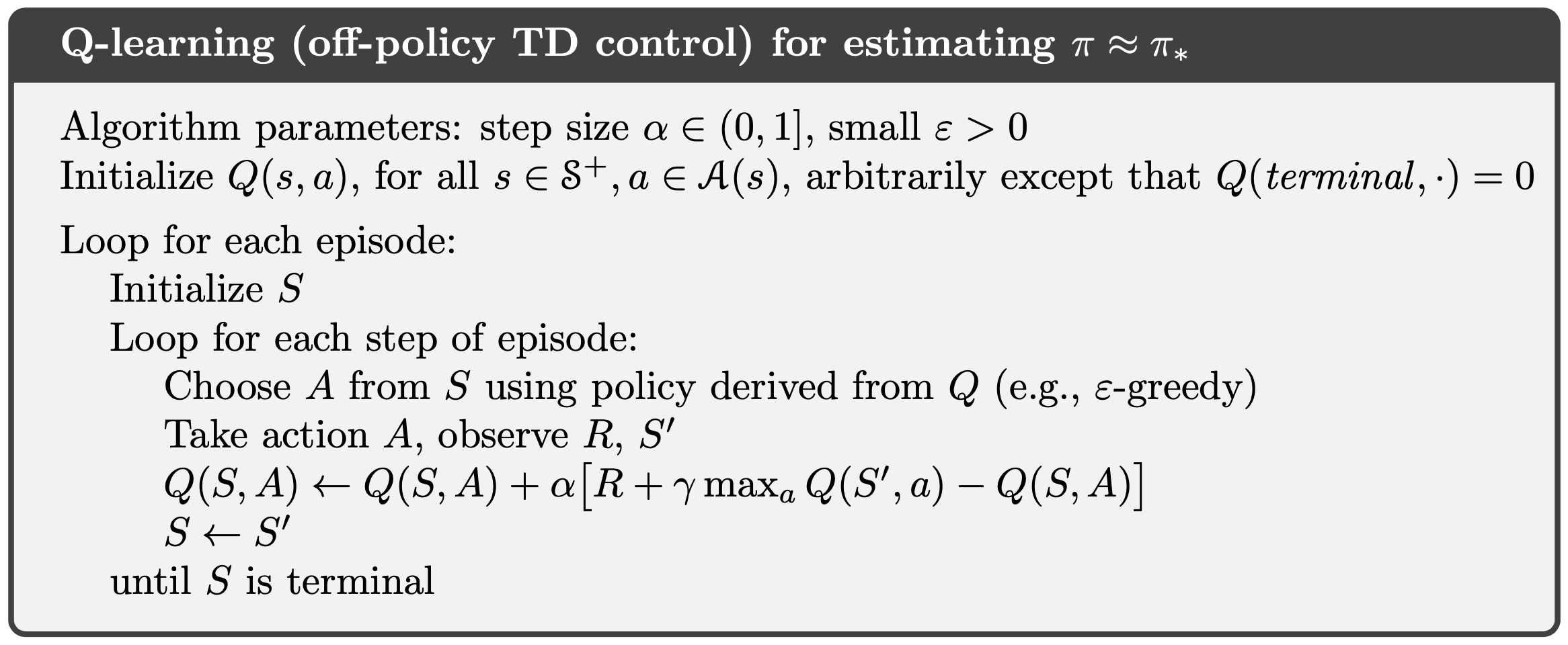
Q Learning
The Q learning (QL) is a TD version of the Q-value iteration. It is the most popular value-based RL algorithm as it naturally uses the off-policy mechanism to update the policy, but without the IS. The QL updates the Q value with respect to the maximum Q value at the next time step. In other words, the greedy policy is used as the target policy.
\[\begin{equation} q_{\pi}^{(i+1)} ( s_{t} , a_{t} ) \leftarrow q_{\pi}^{(i)} ( s_{t} , a_{t} ) + \alpha \left( \hat{q}_{\pi}^{(i)} ( s_{t} , a_{t} ) - q_{\pi}^{(i)} ( s_{t} , a_{t} ) \right) \\ \hat{q}_{\pi}^{(i)} ( s_{t} , a_{t} ) = r_{t+1}^{(\beta)} + \gamma \max_{a'} q^{(i)} ( s_{t+1} , a' ) \equiv r_{t+1}^{(\beta)} + \gamma q_{\pi}^{(i)} ( s_{t+1} , a_{t+1} ) \end{equation}\]- \(\max_{a'} q^{(i)} ( s_{t+1} , a' )\) means that \(a'\) has been sampled in a way that obtains the maximum Q value at \(s_{t+1}\), which is equivalent to using the greedy target policy, so \(\max_{a'} q^{(i)} ( s_{t+1} , a' ) \equiv q_{\pi}^{(i)} ( s_{t+1} , a_{t+1} )\).
- This also means that the QL requires to compute \(q^{(i)} ( s_{t+1} , a' )\) for every \(a' \in \mathcal{A}\) during the update while the TD learning and SARSA do not.
- The IS can be ignored in the QL because:
- \(\max_{a'} q^{(i)} ( s_{t+1} , a' )\) is equivalent to \(\gamma q_{\pi}^{(i)} ( s_{t+1} , a_{t+1} )\) with the greedy policy.
- \(r_{t+1}^{(\beta)}\) is used to update the Q value of the action that acquired the reward.
- Some discussions on stack exchange are Why don’t we use importance sampling for one step Q-learning? and Why we don’t use importance sampling in tabular Q-Learning?.
- The QL follows \(1\)-step bootstrapping, so in theory, if the \(n\)-step is used, the QL also needs the IS. Sutton and Barto introduced the \(n\)-step tree backup algorithm for the \(n\)-step QL, but it seems like small \(n\) without the IS still works in practice, i.e. 3-step in RAINBOW.
The QL pseudocode is:
The QL obtains the optimal value directly, so it is more efficient than the SARSA. However, this introduces additional maximization bias. Since \(\max\) is convex, under the Jensen’s inequality:
\[\begin{align} \mathbb{E}_{ \tau \sim \pi } \left[ \max_{a'} q^{(i)} ( s_{t+1} , a' ) \right] \geq \max_{a'} \mathbb{E}_{ \tau \sim \pi } \left[ q^{(i)} ( s_{t+1} , a' ) \right] \end{align}\]Thus, using the bias definition:
\[\begin{align} b ( \max_{a'} q^{(i)} ( s_{t+1} , a' ) ) & = \mathbb{E}_{ \tau \sim \pi } \left[ \max_{a'} q^{(i)} ( s_{t+1} , a' ) \right] - \max_{a'} q^{(i)} ( s_{t+1} , a' ) \\ & = \mathbb{E}_{ \tau \sim \pi } \left[ \max_{a'} q^{(i)} ( s_{t+1} , a' ) \right] - \max_{a'} \mathbb{E}_{ \tau \sim \pi } \left[ q^{(i)} ( s_{t+1} , a' ) \right] \\ & \geq 0 \end{align}\]This can be easily viewed in the cliff walking problem:
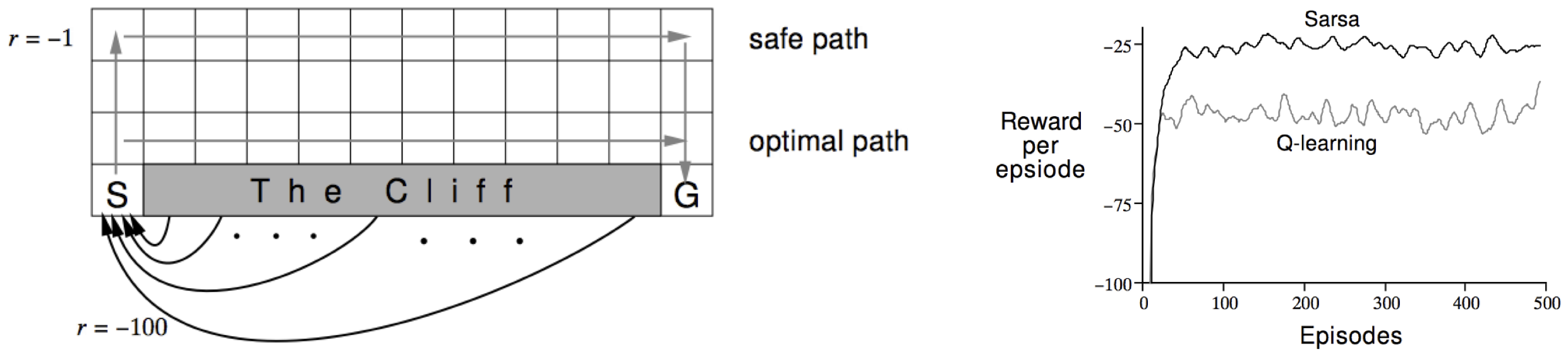
Where The Cliff is the terminal state with the reward of \(-100\), otherwise the reward of \(-1\). The QL always takes the shortest but relatively risky path while the SARSA takes the safe path.
Summary
In this post, the value-based RL algorithms are covered. Their methods are divided into:
- Policy evaluation: A process of evaluating the policy by obtaining the Bellman equation.
- Dynamic Programming: Full & shallow backups, known as model-based. It is not preferred in the real world scenario since it requires to access the environment dynamics.
- Temporal Difference: Sample & shallow backups, known as model-free. It is generally preferred due to its flexibility and simplicity. It is known to have high bias and low variance, but bias and variance can be balanced using n-step bootstrapping.
- Monte Carlo: Sample & deep backups, known as model-free. It is generally less preferred than the temporal difference due to its inflexibility and complexity. It is known to have low bias and high variance.
- Policy improvement: A process of obtaining the improved policy from the Bellman equation.
- Greedy policy: A type of deterministic policy.
- Softmax policy: A type of stochastic policy.
Based on the policy evaluation, the algorithms are divided into:
- Model-based: The optimal policy is obtained using the environment dynamics, such as \(p ( s' \vert s , a )\). DP is known as model-based.
-
Model-free: The optimal policy is obtained using sampled trajectories \(\tau\). TD and MC are known as model-free.
- The update of model-free algorithms can further be generalized as:
- Model-free algorithms are known to suffer from bias and variance problems.
- TD is known to have high bias and low variance
- MC is known to have low bias and high variance.
- To balance bias and variance, the \(n\)-step bootstrapping is often employed.
The value-based RL algorithms are generally divided into:
- Policy Iteration: The policy evaluation with the Bellman expectation equation and the policy improvement.
- Value Iteration: The policy evaluation with the Bellman optimality equation, which encapsulates the policy improvement with the greedy policy.
DP and TD algorithms are:
Where the first and second algorithms are of the policy iteration and the last algorithm is of the value iteration.
In TD, there are two ways to sample \(\tau\).
- On-policy: How the agent explores is the same as what it learns, or \(a \sim \pi ( a \vert s )\) where \(\pi ( a \vert s ) = \arg \max_{a} q_{\pi} ( s , a )\).
- Off-policy: How the agent explores is different from what it learns, or \(a \sim \beta ( a \vert s )\) and \(\pi ( a \vert s ) = \arg \max_{a} q_{\pi} ( s , a )\), where \(\beta ( a \vert s )\) is referred to as the behaviour policy and \(\pi ( a \vert s )\) is referred to as the target policy such that \(\beta ( a \vert s ) \neq \pi ( a \vert s )\).
\(\beta\) is used to act on the environment and collect trajectories while \(\pi\) is the policy updated with the collected trajectories. In general, \(\beta\) uses \(\pi\) partially, either with probability or smoothing.
The off-policy method introduces the distribution shift, where the distribution we are following, \(\beta\), is not the same as the distribution we are updating, \(\pi\). To diminish this effect, we use the IS.
\[\require{color} \begin{align} \hat{q}_{\pi}^{(i)} ( s_{t} , a_{t} ) & = \prod_{l=0}^{\infty} \frac{ \pi ( a_{t+l} \vert s_{t+l} ) } { \beta ( a_{t+l} \vert s_{t+l} ) } \left( \sum_{k=0}^{\infty} \gamma^{k} r_{t+k+1}^{[\beta]} \right) = \prod_{l=0}^{\infty} \frac{ \pi ( a_{t+l} \vert s_{t+l} ) } { \beta ( a_{t+l} \vert s_{t+l} ) } R_{t}^{[\beta]} = R_{t}^{[\pi]} \\ & \equiv \prod_{l=0}^{n-1} \frac{ \pi ( a_{t+l} \vert s_{t+l} ) } { \beta ( a_{t+l} \vert s_{t+l} ) } \left( \sum_{k=0}^{n-1} \gamma^{k} r_{t+k+1}^{[\beta]} + \gamma^{n} q_{\pi}^{(i)} ( s_{t+n} , a_{t+n} ) \right) \end{align}\]The QL is the most popular value-based RL algorithm. In summary, the QL:
- uses sampling, so it is robust to complex unknown environments. (Pros over DP)
- has low variance due to bootstrapping, so it converges fast. (Pros over MC)
- is off-policy, so it has better exploration than on-policy. (Pros over on-policy)
- avoids importance sampling correction since it uses the Bellman optimality equation. (Pros over TD learning and SARSA)
- has initialization bias, so the initialization influences the convergence. (Cons over MC)
- has overestimation bias, so it takes a risky path. (Cons over SARSA)
Reference
- Lecture 3 to 5 of David Silver’s lecture
- Chapter 4 to 7 in Reinforcement Learning: An Introduction
Comments