Policy-based Reinforcement Learning
Machine intelligence is the last invention that humanity will ever need to make.
Nick Bostrom
If the universe is constructed with patterns and humans can interpret this, then so may machines. If machines become intelligent over humans, humans need not apply.
Machine learning is the study of algorithms that involve training a computer to learn patterns and relationships in data without being explicitly programmed. It can be divided into three types:
- Supervised Learning: The algorithm, or model, is trained on labeled data, where the goal is to map each input to the correct output.
- Unsupervised Learning: The algorithm, or model, is trained on unlabeled data, where the goal is to identify patterns or structure in the data without being told what to look for.
- Reinforcement Learning: The algorithm, or agent, is trained on the interactive worlds, where the goal is to learn a policy that maximizes rewards and minimize penalties.
The problems in ML can be largely divided by four types:
- Computer Vision: The problems require machines to interpret and understand visual data, i.e. images and videos. They includes image classification, object localization, video analysis, image captioning and visual question answering.
- Natural Language Processing: The problems require machines to interpret and understand human language, i.e. words and documents. They includes text classification, translation, summarization, speech analysis, question answering and dialogue system.
- Graph Analysis: The problems require machines to interpret and understand graph data, i.e. nodes and edges in graphs. They includes graph classification, link prediction, knowledge graph, social network analysis, recommendation system, combinatorial optimization and path finding.
- Decision Making: The problems require machines to interact with the world and choose an appropriate action based on data and objectives. They include game playing, autonomous vehicles and robotics.
Reinforcement learning is a subfield of machine learning, popular in decision making problems. The algorithms are generally grouped by:
| Value-based | Policy-based | |||
| Model-based | Model-free | |||
| Classic |
Policy Iteration,
Value Iteration |
Monte Carlo,
SARSA,
Q Learning |
Policy Gradient , Deterministic Policy Gradient | |
| Deep |
Deep Q Network, Double Deep Q Network,
Duel Deep Q Network, Rainbow |
Vanilla Policy Gradient, Natural Policy Gradient,
Trust Region Policy Optimization, Proximal Policy Optimization |
||
| Classic | Actor Critic | |||
| Deep |
Deep Deterministic Policy Gradient, Twin Delayed Deep Deterministic Policy Gradient,
Soft Q Learning, Soft Actor Critic |
|||
Policy-based reinforcement learning is one of two fundamental classes of reinforcement learning algorithms. It explicitly constructs the policy, directly mapping from the state to the action, such that maximizes the return. Unlike value-based reinforcement learning, policy-based reinforcement learning attempts directly find the optimal policy by optimizing:
\[\begin{equation} \mathcal{J} ( \theta ) = \mathbb{E}_{ s \sim d^{\pi_{\theta}}, a \sim \pi_{\theta} } [ R ( s , a ) ] \end{equation}\]Where maximizing the objective is to obtain \(\pi_{\theta}\) such that maximizes \(R\) for every \(s\) and \(a\). This post aims to provide a tutorial on policy-based reinforcement learning algorithms and introduce a combination of value-based and policy-based reinforcement learning algorithm.
Policy Gradient
The policy gradient (PG) is an on-policy reinforcement learning (RL) algorithm that finds the optimal policy using the Monte-Carlo (MC) method. Unlike value-based methods, the PG parameterizes the policy with a function approximator such that maximizes the return. This has two advantages over value-based RL algorithms.
- The policy is naturally stochastic.
- The action space can be either discrete or continuous.
Consider the standard RL framework with an agent with the parameterized policy, \(\pi_{\theta}\), where \(\theta\) is the parameter. The optimal policy, \(\pi^{\ast}\), is:
\[\begin{equation} \pi^{\ast} ( a \vert s ) = \arg \max_{\pi} \mathbb{E}_{ s \sim d^{\pi}, a \sim \pi } [ R ( s , a ) ] \end{equation}\]Then, the objective function can be expressed as:
\[\begin{equation} \mathcal{J} ( \theta ) = \mathbb{E}_{ s \sim d^{\pi_{\theta}}, a \sim \pi_{\theta} } [ R ( s , a ) ] \end{equation}\]Maximizing the objective through gradient ascent obtains \(\theta\) that results in the policy which drives the agent to the high expected return at any state-action pair.
- The PG objective is different from \(Q^{\pi_{\theta}} ( s , a ) = \mathbb{E}_{ \tau \sim \pi_{\theta} } [ R_{t} \vert s_{t} = s , a_{t} = a ]\).
- The Q value is the expectation of the return for a particular state-action pair.
- The PG objective is the expectation of the return for any state-action pair.
- If the MDP is average-reward continuous and ergodic, maximizing \(Q^{\pi_{\theta}}\) is actually the same as the PG objective.
The PG objective function has many equivalent expressions.
\[\begin{align} \mathcal{J} ( \theta ) & = \mathbb{E}_{ s \sim d^{\pi_{\theta}}, a \sim \pi_{\theta} } [ R ( s , a ) ] = \sum_{s \in \mathcal{S}} d^{\pi_{\theta}} ( s ) \sum_{a \in \mathcal{A}} \pi_{\theta} (a \vert s) R ( s , a ) \\ & \equiv \mathbb{E}_{ s \sim d^{\pi_{\theta}}, a \sim \pi_{\theta} } \left[ Q^{\pi_{\theta}} (s, a) \right] = \sum_{s \in \mathcal{S}} d^{\pi_{\theta}} ( s ) \sum_{a \in \mathcal{A}} \pi_{\theta} (a \vert s) Q^{\pi_{\theta}} (s, a) \\ & \equiv \mathbb{E}_{ s \sim d^{\pi_{\theta}} } \left[ V^{\pi_{\theta}} (s) \right] = \sum_{s \in \mathcal{S}} d^{\pi_{\theta}} ( s ) V^{\pi_{\theta}} (s) \\ & \equiv \mathbb{E}_{ s_{0} \sim p_{0} } \left[ V^{\pi_{\theta}} (s_{0}) \right] = \sum_{s_{0} \in \mathcal{S}} p_{0} ( s_{0} ) V^{\pi_{\theta}} (s_{0}) \end{align}\]Maximizing any of the expressions leads to the optimal policy.
- Since \(d^{\pi_{\theta}} ( s ) \in [0, 1]\) and \(\pi_{\theta} (a \vert s) \in [0, 1]\), \(\sum_{s \in \mathcal{S}} d^{\pi_{\theta}} ( s ) \sum_{a \in \mathcal{A}} \pi_{\theta} (a \vert s) R ( s , a )\) is the expectation of the \(R\).
- Even if \(Q^{\pi_{\theta}}\) is not the same as the PG objective, acquiring \(\theta\) that maximizes \(Q^{\pi_{\theta}}\) is equivalent to maximizing \(R\).
Policy Gradient Theorem
Computing the gradient of the PG objective, \(\nabla_{\theta} \mathcal{J}\), is very difficult since:
- \(\nabla_{\theta} \left( \sum_{s \in \mathcal{S}} d^{\pi_{\theta}} ( s ) \sum_{a \in \mathcal{A}} \pi_{\theta} (a \vert s) R ( s , a ) \right)\) is intractable because \(d^{\pi_{\theta}} ( s )\), \(\pi_{\theta} (a \vert s)\), \(Q^{\pi_{\theta}} (s, a)\), \(V^{\pi_{\theta}} (s)\) and \(R ( s , a )\) are dependent on \(\theta\).
- \(\nabla_{\theta} R ( s , a )\) where \(s \sim d^{\pi_{\theta}}, a \sim \pi_{\theta}\) is doable because \(Q^{\pi_{\theta}} (s, a)\), \(V^{\pi_{\theta}} (s)\) and \(R ( s , a )\) are not explicit functions of \(\theta\).
The Theorem 1 (Policy Gradient) allows us to approximate \(\nabla_{\theta} \mathcal{J}\) into tractable form.
\[\begin{align} \nabla_{\theta} \mathcal{J} ( \theta ) & = \nabla_{\theta} \sum_{s \in \mathcal{S}} d^{\pi_{\theta}} ( s ) \sum_{a \in \mathcal{A}} \pi_{\theta} (a \vert s) Q^{\pi_{\theta}} (s, a) = \mathbb{E}_{ s \sim d^{\pi_{\theta}}, a \sim \pi_{\theta} } \left[ \nabla_{\theta} Q^{\pi_{\theta}} (s, a) \right] \\ & \propto \sum_{s \in \mathcal{S}} d^{\pi_{\theta}} ( s ) \sum_{a \in \mathcal{A}} \pi_{\theta} (a \vert s) Q^{\pi_{\theta}} (s, a) \nabla_{\theta} \pi_{\theta} (a \vert s) = \mathbb{E}_{ s \sim d^{\pi_{\theta}}, a \sim \pi_{\theta} } \left[ Q^{\pi_{\theta}} (s, a) \nabla_{\theta} \ln \pi_{\theta} (a \vert s) \right] \end{align}\]In the original paper, the theorem is proved in two different environments, start-state episodic and average-reward continuous, but in this post, I will stick with the episodic environment without a discount factor since it is more intuitive and blends well with previous posts.
The gradient of the PG objective can be defined as:
\[\begin{equation} \nabla_{\theta} \mathcal{J} ( \theta ) \equiv \nabla_{\theta} \mathbb{E}_{ s \sim d^{\pi_{\theta}} } \left[ V^{\pi_{\theta}} (s) \right] \equiv \nabla_{\theta} V^{\pi_{\theta}} (s) \quad \forall s \in \mathcal{S} \end{equation}\]We can decompose \(\nabla_{\theta} V^{\pi_{\theta}} ( s )\) into:
\[\require{color} \begin{align} \textcolor{red}{\nabla_{ \theta }} V^{ \pi_{\theta} } (s) = & \textcolor{red}{\nabla_{ \theta }} \left( \sum_{a \in \mathcal{A} } \pi_\theta (a \vert s) Q^{\pi_{\theta}} (s, a) \right) \\ = & \sum_{a \in \mathcal{A}} \left( \bigl( \textcolor{red}{\nabla_{ \theta }} \pi_{\theta} (a \vert s) \bigr) Q^{\pi_{\theta}} (s, a) + \pi_{\theta} (a \vert s) \bigl( \textcolor{red}{\nabla_{ \theta }} Q^{\pi_{\theta}} (s, a) \bigr) \right) \\ = & \sum_{a \in \mathcal{A}} \left( Q^{\pi_{\theta}} (s, a) \textcolor{red}{\nabla_{ \theta }} \pi_{\theta} (a \vert s) + \pi_{\theta} (a \vert s) \left( \textcolor{red}{\nabla_{ \theta }} \sum_{s' \in \mathcal{S}} p(s' \vert s, a) \textcolor{blue}{(r (s, a) + V^{\pi_{\theta}} (s'))} \right) \right) \\ = & \sum_{a \in \mathcal{A}} \left( Q^{\pi_{\theta}} (s, a) \textcolor{red}{\nabla_{ \theta }} \pi_{\theta} (a \vert s) + \pi_{\theta} (a \vert s) \sum_{s' \in \mathcal{S}} p(s' \vert s,a) \textcolor{blue}{} \textcolor{red}{\nabla_{ \theta }} \textcolor{blue}{V^{\pi_{\theta}}(s')} \right) \\ = & \sum_{a \in \mathcal{A}} Q^{\pi_{\theta}} (s, a) \nabla_{ \theta} \pi_{\theta} (a \vert s) + \sum_{a \in \mathcal{A}} \left( \pi_{\theta} (a \vert s) \sum_{s' \in \mathcal{S}} p(s' \vert s,a) \nabla_{ \theta} V^{\pi_{\theta}}(s') \right) \\ = & \sum_{a \in \mathcal{A}} Q^{\pi_{\theta}} (s, a) \nabla_{ \theta} \pi_{\theta} (a \vert s) + \sum_{s' \in \mathcal{S}} \left( \textcolor{red}{\sum_{a \in \mathcal{A}} \pi_{\theta} (a \vert s) p(s' \vert s,a)} \right) \nabla_{ \theta} V^{\pi_{\theta}}(s') \\ = & \sum_{a \in \mathcal{A}} Q^{\pi_{\theta}} (s, a) \nabla_{ \theta} \pi_{\theta} (a \vert s) + \sum_{s' \in \mathcal{S}} \textcolor{blue}{\Pr (s \rightarrow s' \vert 1, \pi_{\theta})} \nabla_{ \theta} V^{\pi_{\theta}}(s') \end{align}\]Where the state visitation probability is \(\textcolor{blue}{\Pr (s \rightarrow s' \vert 1, \pi_{\theta})} = \textcolor{red}{\sum_{a \in \mathcal{A}} \pi_{\theta} (a \vert s) p(s' \vert s,a)}\).
Then, recursively:
\[\require{color} \begin{align} \nabla_{ \theta } V^{ \pi_{\theta} } (\textcolor{red}{s}) = & \sum_{a \in \mathcal{A}} Q^{\pi_{\theta}} (\textcolor{red}{s}, a) \nabla_{ \theta } \pi_{\theta} (a \vert \textcolor{red}{s}) \\ & + \sum_{\textcolor{blue}{s'} \in \mathcal{S}} \Pr (\textcolor{red}{s} \rightarrow \textcolor{blue}{s'} \vert 1, \pi_{\theta}) \nabla_{ \theta} V^{\pi_{\theta}}(\textcolor{blue}{s'}) \\ = & \sum_{a \in \mathcal{A}} Q^{\pi_{\theta}} (\textcolor{red}{s}, a) \nabla_{ \theta } \pi_{\theta} (a \vert \textcolor{red}{s}) \\ & + \sum_{\textcolor{blue}{s'} \in \mathcal{S}} \Pr (\textcolor{red}{s} \rightarrow \textcolor{blue}{s'} \vert 1, \pi_{\theta}) \Biggl( \sum_{a’ \in \mathcal{A}} Q^{\pi_{\theta}} (\textcolor{blue}{s'}, a’) \nabla_{ \theta } \pi_{\theta} (a’ \vert \textcolor{blue}{s'}) + \sum_{\textcolor{green}{s''} \in \mathcal{S}} \Pr (\textcolor{blue}{s'} \rightarrow \textcolor{green}{s''} \vert 1, \pi_{\theta}) \nabla_{ \theta} V^{\pi_{\theta}}(\textcolor{green}{s''}) \Biggr) \\ = & \sum_{a \in \mathcal{A}} Q^{\pi_{\theta}} (\textcolor{red}{s}, a) \nabla_{ \theta } \pi_{\theta} (a \vert \textcolor{red}{s}) \\ & + \sum_{\textcolor{blue}{s'} \in \mathcal{S}} \Pr (\textcolor{red}{s} \rightarrow \textcolor{blue}{s'} \vert 1, \pi_{\theta}) \sum_{a’ \in \mathcal{A}} Q^{\pi_{\theta}} (\textcolor{blue}{s'}, a’) \nabla_{ \theta } \pi_{\theta} (a’ \vert \textcolor{blue}{s'}) \\ & + \sum_{\textcolor{blue}{s'} \in \mathcal{S}} \Pr (\textcolor{red}{s} \rightarrow \textcolor{blue}{s'} \vert 1, \pi_{\theta}) \sum_{\textcolor{green}{s''} \in \mathcal{S}} \Pr (\textcolor{blue}{s'} \rightarrow \textcolor{green}{s''} \vert 1, \pi_{\theta}) \nabla_{ \theta} V^{\pi_{\theta}}(\textcolor{green}{s''}) \\ = & \sum_{a \in \mathcal{A}} Q^{\pi_{\theta}} (\textcolor{red}{s}, a) \nabla_{ \theta } \pi_{\theta} (a \vert \textcolor{red}{s}) \\ & + \sum_{\textcolor{blue}{s'} \in \mathcal{S}} \Pr (\textcolor{red}{s} \rightarrow \textcolor{blue}{s'} \vert 1, \pi_{\theta}) \sum_{a’ \in \mathcal{A}} Q^{\pi_{\theta}} (\textcolor{blue}{s'}, a’) \nabla_{ \theta } \pi_{\theta} (a’ \vert \textcolor{blue}{s'}) \\ & + \sum_{\textcolor{green}{s''} \in \mathcal{S}} \Pr (\textcolor{red}{s} \rightarrow \textcolor{green}{s''} \vert 2, \pi_{\theta}) \nabla_{ \theta} V^{\pi_{\theta}}(\textcolor{green}{s''}) \\ = & \sum_{\textcolor{red}{s} \in \mathcal{S}} \Pr (\textcolor{red}{s} \rightarrow \textcolor{red}{s} \vert 0, \pi_{\theta}) \sum_{a \in \mathcal{A}} Q^{\pi_{\theta}} (\textcolor{red}{s}, a) \nabla_{ \theta } \pi_{\theta} (a \vert \textcolor{red}{s}) \\ & + \sum_{\textcolor{blue}{s'} \in \mathcal{S}} \Pr (\textcolor{red}{s} \rightarrow \textcolor{blue}{s'} \vert 1, \pi_{\theta}) \sum_{a’ \in \mathcal{A}} Q^{\pi_{\theta}} (\textcolor{blue}{s'}, a’) \nabla_{ \theta } \pi_{\theta} (a’ \vert \textcolor{blue}{s'}) \\ & + \sum_{\textcolor{green}{s''} \in \mathcal{S}} \Pr (\textcolor{red}{s} \rightarrow \textcolor{green}{s''} \vert 2, \pi_{\theta}) \sum_{a’’ \in \mathcal{A}} Q^{\pi_{\theta}} (\textcolor{green}{s''}, a'') \nabla_{ \theta } \pi_{\theta} (a'' \vert \textcolor{green}{s''}) + \cdots \\ = & \sum_{\textcolor{violet}{x} \in \mathcal{S}} \sum_{\textcolor{orange}{k} = 0}^{\infty} \Pr (\textcolor{red}{s} \rightarrow \textcolor{violet}{x} \vert \textcolor{orange}{k}, \pi_{\theta}) \sum_{a \in \mathcal{A}} Q^{\pi_{\theta}} (\textcolor{violet}{x}, a) \nabla_{ \theta } \pi_{\theta} (a \vert \textcolor{violet}{x}) \end{align}\]Finally, the update is:
\[\begin{align} \nabla_{ \theta } \mathcal{J} (\theta) \equiv & \sum_{\textcolor{red}{s_{0}} \in \mathcal{S}} p ( \textcolor{red}{s_{0}} ) \nabla_{ \theta } V^{ \pi_{\theta} } (\textcolor{red}{s_{0}}) \\ = & \sum_{\textcolor{red}{s_{0}} \in \mathcal{S}} p ( \textcolor{red}{s_{0}} ) \sum_{\textcolor{blue}{s} \in \mathcal{S}} \sum_{\textcolor{orange}{k} = 0}^{\infty} \Pr (\textcolor{red}{s_{0}} \rightarrow \textcolor{blue}{s} \vert \textcolor{orange}{k}, \pi_{\theta}) \sum_{a \in \mathcal{A}} Q^{\pi_{\theta}} (\textcolor{blue}{s}, a) \nabla_{ \theta } \pi_{\theta} (a \vert \textcolor{blue}{s}) \\ = & \sum_{\textcolor{blue}{s} \in \mathcal{S}} \left( \sum_{\textcolor{red}{s_{0}} \in \mathcal{S}} \sum_{\textcolor{orange}{k} = 0}^{\infty} p ( \textcolor{red}{s_{0}} ) \Pr (\textcolor{red}{s_{0}} \rightarrow \textcolor{blue}{s} \vert \textcolor{orange}{k}, \pi_{\theta}) \right) \sum_{a \in \mathcal{A}} Q^{\pi_{\theta}} (\textcolor{blue}{s}, a) \nabla_{ \theta } \pi_{\theta} (a \vert \textcolor{blue}{s}) \\ = & \sum_{\textcolor{blue}{s} \in \mathcal{S}} d^{\pi_{\theta}} ( \textcolor{blue}{s} ) \sum_{a \in \mathcal{A}} Q^{\pi_{\theta}} (\textcolor{blue}{s}, a) \nabla_{ \theta} \pi_{\theta} (a \vert \textcolor{blue}{s}) \\ = & \sum_{s \in \mathcal{S}} d^{\pi_{\theta}} ( s ) \sum_{a \in \mathcal{A}} \frac{ \pi_{\theta} (a \vert s) }{\pi_{\theta} (a \vert s)} Q^{\pi_{\theta}} (s, a) \nabla_{ \theta} \pi_{\theta} (a \vert s) \\ = & \sum_{s \in \mathcal{S}} d^{\pi_{\theta}} ( s ) \sum_{a \in \mathcal{A}} \pi_{\theta} (a \vert s) Q^{\pi_{\theta}} (s, a) \frac{ \nabla_{ \theta} \pi_{\theta} (a \vert s) }{\pi_{\theta} (a \vert s)} \\ = & \sum_{s \in \mathcal{S}} d^{\pi_{\theta}} ( s ) \sum_{a \in \mathcal{A}} \pi_{\theta} (a \vert s) Q^{\pi_{\theta}} (s, a) \nabla_{ \theta} \ln \pi_{\theta} (a \vert s) = \mathbb{E}_{ s \sim d^{\pi_{\theta}}, a \sim \pi_{\theta} } \left[ Q^{\pi_{\theta}} (s, a) \nabla_{ \theta} \ln \pi_{\theta} (a \vert s) \right] \end{align}\]Another way to view the PG objective is from the log-likelihood. The PG objective without the value function is actually the same as the objective used in the behavioral cloning in imitation learning and more generally the log-likelihood in supervised learning. In the behavioral cloning, there are two factors that determine the policy:
- The representation of the demonstrations in the dataset
- The sampling distribution of the demonstrations from the dataset
If the sampling distribution is skewed for the update, the agent will learn the representations of the demonstration data that are more frequently sampled. On the other hand, the PG contains the value function in its objective. This enforces the agent to learn from:
- The representation of the experiences
- The sampling distribution of the experiences which is determined by the exploration
- The value function as the magnitude of the acquired experiences
Thus, what the value function does is that it acts as the magnitude on how important the experience is. This will be discussed in later posts.
Policy Gradient with Function Approximation
The use of the real Q value results in high variance since it uses MC to construct the Q value. To reduce this variance, we can use another function approximator for Q value with parameter \(\phi\), where \(Q_{\phi} : \mathcal{S} \times \mathcal{A} \rightarrow \mathbb{R}\), under the Theorem 2 (Policy Gradient with Function Approximation), which deals with two conditions:
\[\begin{equation} \nabla_{ \phi } Q_{ \phi } (s, a) = \nabla_{ \theta} \ln \pi_{\theta} (a \vert s) \qquad \nabla_{ \phi } \mathcal{J} ( \phi ) = \mathbb{E}_{ s \sim d^{\pi_{\theta}} , a \sim \pi_{\theta} } \left[ \left( Q_{\phi} (s, a) - Q^{\pi_{\theta}} (s, a) \right)^{2} \right] \leq \varepsilon \end{equation}\]Where \(\varepsilon\) is a small real number.
- The first condition is that the gradient of the estimated Q value, \(\nabla_{ \phi } Q_{ \phi } (s, a)\), must be equal to \(\nabla_{ \theta} \ln \pi_{\theta} (a \vert s)\).
- The second is that \(Q_{\phi} (s, a)\) must be optimized with the mean squared error with respect to \(Q^{\pi_{\theta}} (s, a)\).
This is actually outside of the scope of the PG since this introduces the value-based method into the policy-based method. However, since the original paper proves this, here it goes. The objective of the Q value can be expressed as:
\[\begin{align} \nabla_{ \phi } \mathcal{J} ( \phi ) = & \nabla_{ \phi } \mathbb{E}_{ s \sim d^{\pi_{\theta}} , a \sim \pi_{\theta} } \left[ \left( Q_{ \phi } (s, a) - Q^{\pi_{\theta}} (s, a) \right)^{2} \right] = \nabla_{ \phi } \varepsilon= 0 \\ = & \nabla_{ \phi } \sum_{s \in \mathcal{S}} d^{\pi_{\theta}} ( s ) \sum_{a \in \mathcal{A}} \pi_{\theta} (a \vert s) \left( Q_{ \phi } (s, a) - Q^{\pi_{\theta}} (s, a) \right)^{2} \\ = & \sum_{s \in \mathcal{S}} d^{\pi_{\theta}} ( s ) \sum_{a \in \mathcal{A}} \pi_{\theta} (a \vert s) \cdot 2 \left( Q_{ \phi } (s, a) - Q^{\pi_{\theta}} (s, a) \right) \nabla_{ \phi } Q_{ \phi } (s, a) \\ \propto & \sum_{s \in \mathcal{S}} d^{\pi_{\theta}} ( s ) \sum_{a \in \mathcal{A}} \pi_{\theta} (a \vert s) \left( Q_{ \phi } (s, a) - Q^{\pi_{\theta}} (s, a) \right) \nabla_{ \phi } Q_{ \phi } (s, a) \quad \nabla_{ \phi } Q_{ \phi } (s, a) = \nabla_{ \theta} \ln \pi_{\theta} (a \vert s) \\ = & \sum_{s \in \mathcal{S}} d^{\pi_{\theta}} ( s ) \sum_{a \in \mathcal{A}} \pi_{\theta} (a \vert s) \left( Q_{ \phi } (s, a) - Q^{\pi_{\theta}} (s, a) \right) \nabla_{ \theta} \ln \pi_{\theta} (a \vert s) \\ = & \sum_{s \in \mathcal{S}} d^{\pi_{\theta}} ( s ) \sum_{a \in \mathcal{A}} \pi_{\theta} (a \vert s) Q_{ \phi } (s, a) \nabla_{ \theta} \ln \pi_{\theta} (a \vert s) - \sum_{s \in \mathcal{S}} d^{\pi_{\theta}} ( s ) \sum_{a \in \mathcal{A}} \pi_{\theta} (a \vert s) Q^{\pi_{\theta}} (s, a) \nabla_{ \theta} \ln \pi_{\theta} (a \vert s) = 0 \end{align}\]This means:
\[\begin{align} \sum_{s \in \mathcal{S}} d^{\pi_{\theta}} ( s ) \sum_{a \in \mathcal{A}} \pi_{\theta} (a \vert s) Q_{ \phi } (s, a) \nabla_{ \theta} \ln \pi_{\theta} (a \vert s) & = \sum_{s \in \mathcal{S}} d^{\pi_{\theta}} ( s ) \sum_{a \in \mathcal{A}} \pi_{\theta} (a \vert s) Q^{\pi_{\theta}} (s, a) \nabla_{ \theta} \ln \pi_{\theta} (a \vert s) \\ \mathbb{E}_{ s \sim d^{\pi_{\theta}} , a \sim \pi_{\theta} } \left[ Q_{ \phi } (s, a) \nabla_{ \theta} \ln \pi_{\theta} (a \vert s) \right] & = \mathbb{E}_{ s \sim d^{\pi_{\theta}} , a \sim \pi_{\theta} } \left[ Q^{\pi_{\theta}} (s, a) \nabla_{ \theta} \ln \pi_{\theta} (a \vert s) \right] \end{align}\]Therefore, 1) if \(\nabla_{ \phi } Q_{ \phi } (s, a) = \nabla_{ \theta} \ln \pi_{\theta} (a \vert s)\) holds and 2) if the function approximation of \(Q_{ \phi }\) is optimized with the mean squared error with \(Q^{\pi_{\theta}}\), we can set the objective function as:
\[\begin{equation} \nabla_{ \theta } \mathcal{J} (\theta) \propto \mathbb{E}_{ s \sim d^{\pi_{\theta}} , a \sim \pi_{\theta} } \left[ Q^{\pi_{\theta}} (s, a) \nabla_{ \theta} \ln \pi_{\theta} (a \vert s) \right] \equiv \mathbb{E}_{ s \sim d^{\pi_{\theta}} , a \sim \pi_{\theta} } \left[ Q_{ \phi } (s, a) \nabla_{ \theta} \ln \pi_{\theta} (a \vert s) \right] \end{equation}\]In traditional PG, the policy distribution is constructed with parameter, \(\theta\), and a feature vector of state-action pair, \(\mathbf{x} ( s , a )\), where \(\theta, \mathbf{x} ( s , a ) \in \mathbb{R}^{n}\).
Consider a cartpole problem with two state features, \(( x_{p} , x_{v} )\) as (Position, Velocity), and two actions, \(( a_{l} , a_{r} )\) as (Left, Right). The simplest form of \(\mathbf{x} ( s , a )\) can be expressed as:
\[\begin{equation} \mathbf{x} ( s , a = a_{l} ) = \begin{bmatrix} x_{p} & x_{v} & 0 & 0 \end{bmatrix} \qquad \mathbf{x} ( s , a = a_{r} ) = \begin{bmatrix} 0 & 0 & x_{p} & x_{v} \end{bmatrix} \qquad \theta = \begin{bmatrix} \theta_{pl} & \theta_{vl} & \theta_{pr} & \theta_{vr} \end{bmatrix}^{\intercal} \end{equation}\]For a given \(\theta\), parameterized policy will be:
\[\begin{equation} \pi_{\theta} (a_{l} \vert s) = \mathbf{x} ( s , a = a_{l} ) \cdot \theta \qquad \pi_{\theta} (a_{r} \vert s) = \mathbf{x} ( s , a = a_{r} ) \cdot \theta \end{equation}\]Thus, the first two values of \(\theta\) learn to map features to \(a_{l}\) and the last two map features to \(a_{r}\). However, \(\theta\) and \(\mathbf{x}\) are the design choice, so based on the problems and algorithms, they vary.
There are two types of policy distribution that meet the two conditions in the Theorem 2 (Policy Gradient with Function Approximation).
-
Softmax policy distribution: A Gibbs distribution in a linear combination of features, a.k.a. softmax policy distribution, to produce action probability for discrete action space.
\[\begin{equation} \pi_{\theta} (a \vert s) = \text{Softmax} ( e^{ \mathbf{x} ( s , a ) \cdot \theta } ) = \frac{ e^{ \mathbf{x} ( s , a ) \cdot \theta } }{ \sum_{ a' \in \mathcal{A} } e^{ \mathbf{x} ( s , a' ) \cdot \theta } } \end{equation}\]- Where softmax signifies the normalization of \(e^{ \mathbf{x} ( s , a ) \cdot \theta }\) across all the actions. To meet the condition in the Theorem 2 (Policy Gradient with Function Approximation):
- Where \(\theta, \mathbf{x} \in \mathbb{R}^{n}\). Thus, Q value is parameterized with \(\phi \in \mathbb{R}^{n}\).
-
Gaussian policy distribution: A Gaussian distribution with a parameterized mean and a fixed standard deviation for continuous action space.
\[\begin{equation} \pi_{\theta} (a \vert s) = \mathcal{N} ( \mu ( s , a ) , \sigma^{2} ) \quad \mu ( s , a ) = \mathbf{x} ( s , a ) \cdot \theta \end{equation}\]- Where \(\mu\) is the parameterized mean of Gaussian distribution and \(\sigma\) is the fixed standard deviation. To meet the condition in the Theorem 2 (Policy Gradient with Function Approximation):
- Where \(\theta, \mathbf{x} \in \mathbb{R}^{n}\). Thus, Q value is parameterized with \(\phi \in \mathbb{R}^{n}\).
In both cases, the agent samples action from the policy distribution \(a \sim \pi_{\theta} (a \vert s)\).
Deterministic Policy Gradient
The standard stochastic PG with the continuous action space requires integrating over both state and action spaces.
\[\begin{equation} \nabla_{ \theta } \mathcal{J} (\theta) \propto \int_{\mathcal{S}} d^{\pi_{\theta}} ( s ) \int_{\mathcal{A}} \pi_{\theta} (a \vert s) Q^{\pi_{\theta}} (s, a) \nabla_{ \theta} \ln \pi_{\theta} (a \vert s) \text{ d}a \text{ d}s = \mathbb{E}_{ s \sim d^{\pi_{\theta}} , a \sim \pi_{\theta} } \left[ Q^{\pi_{\theta}} (s, a) \nabla_{ \theta} \ln \pi_{\theta} (a \vert s) \right] \end{equation}\]To increase the computational efficiency, the deterministic policy gradient (DPG) is proposed, where the policy is no longer distribution, but just value in the continuous action space. Thus, instead of forming the Gaussian policy to sample actions, \(a \sim \mathcal{N} ( \mu ( s ) , \sigma^{2} )\), we treat the policy as the action, \(a = \mu ( s )\), or the greedy policy in the continuous action space. This allows the objective to be formalized to only integrate over the state space:
\[\begin{align} \mathcal{J} ( \theta ) & = \mathbb{E}_{ s \sim d^{\mu_{\theta}} } [ R ( s , \mu_{\theta} ( s ) ) ] = \int_{\mathcal{S}} d^{\mu_{\theta}} ( s ) R ( s , \mu_{\theta} ( s ) ) \text{ d}s \\ & \equiv \mathbb{E}_{ s \sim d^{\mu_{\theta}} } \left[ Q^{\mu_{\theta}} (s, \mu_{\theta} ( s )) \right] = \int_{\mathcal{S}} d^{\mu_{\theta}} ( s ) Q^{\mu_{\theta}} (s, \mu_{\theta} ( s )) \text{ d}s \\ & \equiv \mathbb{E}_{ s \sim d^{\mu_{\theta}} } \left[ V^{\mu_{\theta}} (s) \right] = \int_{\mathcal{S}} d^{\mu_{\theta}} ( s ) V^{\mu_{\theta}} (s) \text{ d}s \\ & \equiv \mathbb{E}_{ s_{0} \sim p_{0} } \left[ V^{\mu_{\theta}} (s_{0}) \right] = \int_{\mathcal{S}} p_{0} ( s_{0} ) V^{\mu_{\theta}} (s_{0}) \text{ d}s_{0} \end{align}\]Few things to note are:
- The reason why the DPG is more computationally efficient is because the computation is independent of the action space.
- To avoid deficient exploration, the DPG is often implemented as off-policy with the behaviour policy, \(a \sim \beta ( a \vert s ) = \mathcal{N} ( \mu ( s ) , \sigma^{2} )\).
- In other words, the DPG updates the deterministic policy with the trajectories collected by the stochastic policy.
- The original paper used \(\mu ( s )\) notation instead of \(\mu ( s , a )\) to generalize its applications.
Deterministic Policy Gradient Theorem
The Theorem 1 (Deterministic Policy Gradient Theorem) allows us to approximate \(\nabla_{\theta} \mathcal{J}\) into tractable form.
\[\begin{align} \nabla_{\theta} \mathcal{J} ( \theta ) & = \nabla_{\theta} \int_{\mathcal{S}} d^{\mu_{\theta}} ( s ) Q^{\mu_{\theta}} (s, \mu_{\theta} ( s )) \text{ d}s = \mathbb{E}_{ s \sim d^{\mu_{\theta}} } \left[ \nabla_{\theta} Q^{\mu_{\theta}} (s, \mu_{\theta} ( s )) \right] \\ & \propto \int_{\mathcal{S}} d^{\mu_{\theta}} ( s ) \nabla_{ \theta} \mu_{\theta} ( s ) \nabla_{ a } Q^{\mu_{\theta}} (s, a) \vert_{a = \mu_{\theta} ( s )} \text{ d}s = \mathbb{E}_{ s \sim d^{\mu_{\theta}} } \left[ \nabla_{ \theta} \mu_{\theta} ( s ) \nabla_{ a } Q^{\mu_{\theta}} (s, a) \vert_{a = \mu_{\theta} ( s )} \right] \end{align}\]Of course, you can simply apply the chain rule, \(\nabla_{\theta} Q^{\mu_{\theta}} (s, \mu_{\theta} ( s )) = \nabla_{ \theta} \mu_{\theta} ( s ) \nabla_{ a } Q^{\mu_{\theta}} (s, a) \vert_{a = \mu_{\theta} ( s )}\), but the original paper proves this in a similar manner to the PG paper.
The gradient of the DPG objective can be defined as:
\[\begin{equation} \nabla_{\theta} \mathcal{J} ( \theta ) \equiv \nabla_{\theta} \mathbb{E}_{ s \sim d^{\mu_{\theta}} } \left[ V^{\mu_{\theta}} (s) \right] \equiv \nabla_{\theta} V^{\mu_{\theta}} (s) \quad \forall s \in \mathcal{S} \end{equation}\]We can decompose \(\nabla_{\theta} V^{\mu_{\theta}} ( s )\) into:
\[\begin{align} \textcolor{red}{\nabla_{ \theta }} V^{ \mu_{\theta} } (s) = & \textcolor{red}{\nabla_{ \theta }} Q^{\mu_{\theta}} (s, \mu_{\theta} (s)) \\ = & \textcolor{red}{\nabla_{ \theta }} \left( \int_{\mathcal{S}} p(s' \vert s, \mu_{\theta} ( s )) \left( r ( s , \mu_{\theta} ( s ) ) + V^{\mu_{\theta}} (s') \right) \text{ d}s' \right) \\ = & \textcolor{red}{\nabla_{ \theta }} r ( s , \mu_{\theta} ( s ) ) + \textcolor{red}{\nabla_{ \theta }} \int_{\mathcal{S}} p(s' \vert s, \mu_{\theta} ( s )) V^{\mu_{\theta}} (s') \text{ d}s' \\ = & \textcolor{red}{\nabla_{ \theta }} \mu_{\theta} ( s ) \textcolor{blue}{\nabla_{ a }} r ( s , a ) \vert_{a = \mu_{\theta} ( s )} \\ & + \int_{\mathcal{S}} \left( \textcolor{red}{\nabla_{ \theta }} p(s' \vert s, \mu_{\theta} ( s )) \right) V^{\mu_{\theta}} (s') + p(s' \vert s, \mu_{\theta} ( s )) \left( \textcolor{red}{\nabla_{ \theta }} V^{\mu_{\theta}} (s') \right) \text{ d}s' \\ = & \textcolor{red}{\nabla_{ \theta }} \mu_{\theta} ( s ) \textcolor{blue}{\nabla_{ a }} r ( s , a ) \vert_{a = \mu_{\theta} ( s )} \\ & + \int_{\mathcal{S}} V^{\mu_{\theta}} (s') \textcolor{red}{\nabla_{ \theta }} \mu_{\theta} ( s ) \textcolor{blue}{\nabla_{ a }} p(s' \vert s, a) \vert_{a = \mu_{\theta} ( s )} + p(s' \vert s, \mu_{\theta} ( s )) \textcolor{red}{\nabla_{ \theta }} V^{\mu_{\theta}} (s') \text{ d}s' \\ = & \textcolor{red}{\nabla_{ \theta }} \mu_{\theta} ( s ) \textcolor{blue}{\nabla_{ a }} \left. \left( r ( s , a ) + \int_{\mathcal{S}} V^{\mu_{\theta}} (s') p(s' \vert s, a) \text{ d}s' \right) \right\vert_{a = \mu_{\theta} ( s )} + \int_{\mathcal{S}} p(s' \vert s, \mu_{\theta} ( s )) \textcolor{red}{\nabla_{ \theta }} V^{\mu_{\theta}} (s') \text{ d}s' \\ = & \textcolor{red}{\nabla_{ \theta }} \mu_{\theta} ( s ) \textcolor{blue}{\nabla_{ a }} Q^{ \mu_{\theta} } ( s , a ) \vert_{a = \mu_{\theta} ( s )} + \int_{\mathcal{S}} \Pr (s \rightarrow s' \vert 1 , \mu_{\theta} ( s )) \textcolor{red}{\nabla_{ \theta }} V^{\mu_{\theta}} (s') \text{ d}s' \end{align}\]Then, recursively:
\[\begin{align} \textcolor{red}{\nabla_{ \theta }} V^{ \mu_{\theta} } (s) = & \textcolor{red}{\nabla_{ \theta }} \mu_{\theta} ( s ) \textcolor{blue}{\nabla_{ a }} Q^{ \mu_{\theta} } ( s , a ) \vert_{a = \mu_{\theta} ( s )} \\ & + \int_{\mathcal{S}} \Pr (s \rightarrow s' \vert 1 , \mu_{\theta}) \textcolor{red}{\nabla_{ \theta }} V^{\mu_{\theta}} (s') \text{ d}s' \\ = & \textcolor{red}{\nabla_{ \theta }} \mu_{\theta} ( s ) \textcolor{blue}{\nabla_{ a }} Q^{ \mu_{\theta} } ( s , a ) \vert_{a = \mu_{\theta} ( s )} \\ & + \int_{\mathcal{S}} \Pr (s \rightarrow s' \vert 1 , \mu_{\theta}) \left( \textcolor{red}{\nabla_{ \theta }} \mu_{\theta} ( s' ) \textcolor{blue}{\nabla_{ a' }} Q^{ \mu_{\theta} } ( s' , a' ) \vert_{a' = \mu_{\theta} ( s' )} + \int_{\mathcal{S}} \Pr (s' \rightarrow s'' \vert 1 , \mu_{\theta}) \textcolor{red}{\nabla_{ \theta }} V^{\mu_{\theta}} (s'') \text{ d}s'' \right) \text{ d}s' \\ = & \textcolor{red}{\nabla_{ \theta }} \mu_{\theta} ( s ) \textcolor{blue}{\nabla_{ a }} Q^{ \mu_{\theta} } ( s , a ) \vert_{a = \mu_{\theta} ( s )} \\ & + \int_{\mathcal{S}} \Pr (s \rightarrow s' \vert 1 , \mu_{\theta}) \textcolor{red}{\nabla_{ \theta }} \mu_{\theta} ( s' ) \textcolor{blue}{\nabla_{ a' }} Q^{ \mu_{\theta} } ( s' , a' ) \vert_{a' = \mu_{\theta} ( s' )} \text{ d}s' \\ & + \int_{\mathcal{S}} \Pr (s \rightarrow s' \vert 1 , \mu_{\theta}) \int_{\mathcal{S}} \Pr (s' \rightarrow s'' \vert 1 , \mu_{\theta}) \textcolor{red}{\nabla_{ \theta }} V^{\mu_{\theta}} (s'') \text{ d}s'' \text{ d}s' \\ = & \textcolor{red}{\nabla_{ \theta }} \mu_{\theta} ( s ) \textcolor{blue}{\nabla_{ a }} Q^{ \mu_{\theta} } ( s , a ) \vert_{a = \mu_{\theta} ( s )} \\ & + \int_{\mathcal{S}} \Pr (s \rightarrow s' \vert 1 , \mu_{\theta}) \textcolor{red}{\nabla_{ \theta }} \mu_{\theta} ( s' ) \textcolor{blue}{\nabla_{ a' }} Q^{ \mu_{\theta} } ( s' , a' ) \vert_{a' = \mu_{\theta} ( s' )} \text{ d}s' \\ & + \int_{\mathcal{S}} \Pr (s \rightarrow s'' \vert 2 , \mu_{\theta}) \textcolor{red}{\nabla_{ \theta }} V^{\mu_{\theta}} (s'') \text{ d}s'' \\ = & \int_{\mathcal{S}} \Pr (s \rightarrow s \vert 0 , \mu_{\theta}) \textcolor{red}{\nabla_{ \theta }} \mu_{\theta} ( s ) \textcolor{blue}{\nabla_{ a }} Q^{ \mu_{\theta} } ( s , a ) \vert_{a = \mu_{\theta} ( s )} \text{ d}s \\ & + \int_{\mathcal{S}} \Pr (s \rightarrow s' \vert 1 , \mu_{\theta}) \textcolor{red}{\nabla_{ \theta }} \mu_{\theta} ( s' ) \textcolor{blue}{\nabla_{ a' }} Q^{ \mu_{\theta} } ( s' , a' ) \vert_{a' = \mu_{\theta} ( s' )} \text{ d}s' \\ & + \int_{\mathcal{S}} \Pr (s \rightarrow s'' \vert 2 , \mu_{\theta}) \textcolor{red}{\nabla_{ \theta }} \mu_{\theta} ( s'' ) \textcolor{blue}{\nabla_{ a'' }} Q^{ \mu_{\theta} } ( s'' , a'' ) \vert_{a'' = \mu_{\theta} ( s'' )} \text{ d}s'' + \cdots \\ = & \int_{\mathcal{S}} \sum_{k=0}^{\infty} \Pr (s \rightarrow x \vert k , \mu_{\theta}) \textcolor{red}{\nabla_{ \theta }} \mu_{\theta} ( x ) \textcolor{blue}{\nabla_{ a }} Q^{ \mu_{\theta} } ( x , a ) \vert_{a = \mu_{\theta} ( x )} \text{ d}x \end{align}\]Finally, the update is:
\[\begin{align} \nabla_{ \theta } \mathcal{J} ( \theta ) = & \int_{\mathcal{S}} p ( s_{0} ) \nabla_{ \theta } V^{ \mu_{\theta} } ( s_{0} ) \text{ d}s_{0} \\ = & \int_{\mathcal{S}} p ( s_{0} ) \int_{\mathcal{S}} \sum_{k=0}^{\infty} \Pr (s_{0} \rightarrow s \vert k , \mu_{\theta}) \nabla_{ \theta } \mu_{\theta} ( s ) \nabla_{ a } Q^{ \mu_{\theta} } ( s , a ) \vert_{a = \mu_{\theta} ( s )} \text{ d}s \text{ d}s_{0} \\ = & \int_{\mathcal{S}} \left( \int_{\mathcal{S}} \sum_{k=0}^{\infty} p ( s_{0} ) \Pr (s_{0} \rightarrow s \vert k , \mu_{\theta}) \text{ d}s_{0} \right) \nabla_{ \theta } \mu_{\theta} ( s ) \nabla_{ a } Q^{ \mu_{\theta} } ( s , a ) \vert_{a = \mu_{\theta} ( s )} \text{ d}s \\ = & \int_{\mathcal{S}} d^{\mu_{\theta}} ( s ) \nabla_{ \theta } \mu_{\theta} ( s ) \nabla_{ a } Q^{ \mu_{\theta} } ( s , a ) \vert_{a = \mu_{\theta} ( s )} \text{ d}s = \mathbb{E}_{ s \sim d^{\mu_{\theta}} ( s ) } \left[ \nabla_{ \theta} \mu_{\theta} ( s ) \nabla_{ a } Q^{ \mu_{\theta} } (s, a) \vert_{a = \mu_{\theta} ( s )} \right] \end{align}\]The DPG can be seen as the PG with zero standard deviation.
\[\begin{equation} \lim_{\sigma \rightarrow 0} \nabla_{\theta} \mathcal{J} ( \pi_{ \mu_{\theta}, \sigma } ) = \nabla_{\theta} \mathcal{J} ( \mu_{\theta} ) \end{equation}\]- This is the Theorem 2 (Limit of the Stochastic Policy Gradient), which is not proven in this post.
testing
Compatible Function Approximation
Similar to the PG, the DPG also provides a proof of the compatibility of a function approximator for the Q value under the Theorem 3 (Compatible Function Approximation). In the DPG, we use function approximator for \(\nabla_{ a } Q_{ \phi } (s, a) \vert_{a = \mu_{\theta} ( s )}\) instead of \(Q_{\phi} (s, a)\). The two conditions are:
\[\begin{equation} \nabla_{ a } Q_{\phi} (s, a) \vert_{a = \mu_{\theta} ( s )} = \nabla_{ \theta} \mu_{\theta} ( s ) \cdot \phi \qquad \mathcal{J} ( \phi ) = \mathbb{E}_{ s \sim d^{\mu_{\theta}}} \left[ \left( \nabla_{ a } Q_{\phi} (s, a) \vert_{a = \mu_{\theta} ( s )} - \nabla_{ a } Q^{\mu_{\theta}} (s, a) \vert_{a = \mu_{\theta} ( s )} \right)^{2} \right] \leq \varepsilon \end{equation}\]Where \(\varepsilon\) is a small real number.
- The first condition is that the gradient of the estimated Q value for the greedy policy, \(\nabla_{ a } Q_{\phi} (s, a) \vert_{a = \mu_{\theta} ( s )}\), must be equal to \(\nabla_{ \theta} \mu_{\theta} ( s ) \cdot \phi\).
- The second is that \(\nabla_{ a } Q_{\phi} (s, a) \vert_{a = \mu_{\theta} ( s )}\) must be optimized with the mean squared error with respect to \(\nabla_{ a } Q^{\mu_{\theta}} (s, a) \vert_{a = \mu_{\theta} ( s )}\).
Since a function approximator does not estimate the Q value, this is not really the value-based method, but rather a unique method that the DPG has. The objective of the gradient of the Q value can be expressed as:
\[\begin{align} \nabla_{ \phi } \mathcal{J} ( \phi ) = & \nabla_{ \phi } \mathbb{E}_{ s \sim d^{\mu_{\theta}}} \left[ \left( \nabla_{ a } Q_{\phi} (s, a) \vert_{a = \mu_{\theta} ( s )} - \nabla_{ a } Q^{\mu_{\theta}} (s, a) \vert_{a = \mu_{\theta} ( s )} \right)^{2} \right] = \nabla_{ \phi } \varepsilon = 0 \\ = & \nabla_{ \phi } \int_{\mathcal{S}} d^{\mu_{\theta}} ( s ) \left( \nabla_{ a } Q_{\phi} (s, a) \vert_{a = \mu_{\theta} ( s )} - \nabla_{ a } Q^{\mu_{\theta}} (s, a) \vert_{a = \mu_{\theta} ( s )} \right)^{2} \text{ d}s \\ = & \int_{\mathcal{S}} d^{\mu_{\theta}} ( s ) \cdot 2 \left( \nabla_{ a } Q_{\phi} (s, a) \vert_{a = \mu_{\theta} ( s )} - \nabla_{ a } Q^{\mu_{\theta}} (s, a) \vert_{a = \mu_{\theta} ( s )} \right) \nabla_{ \phi } \nabla_{ a } Q_{\phi} (s, a) \vert_{a = \mu_{\theta} ( s )} \text{ d}s \\ \propto & \int_{\mathcal{S}} d^{\mu_{\theta}} ( s ) \left( \nabla_{ a } Q_{\phi} (s, a) \vert_{a = \mu_{\theta} ( s )} - \nabla_{ a } Q^{\mu_{\theta}} (s, a) \vert_{a = \mu_{\theta} ( s )} \right) \nabla_{ \phi } \nabla_{ a } Q_{\phi} (s, a) \vert_{a = \mu_{\theta} ( s )} \text{ d}s \\ & \begin{aligned} \qquad \qquad \qquad \qquad \qquad \qquad \qquad \qquad \qquad \nabla_{ a } Q_{\phi} (s, a) \vert_{a = \mu_{\theta} ( s )} = \nabla_{ \theta} \mu_{\theta} ( s ) \cdot \phi \end{aligned} \\ = & \int_{\mathcal{S}} d^{\mu_{\theta}} ( s ) \left( \nabla_{ a } Q_{\phi} (s, a) \vert_{a = \mu_{\theta} ( s )} - \nabla_{ a } Q^{\mu_{\theta}} (s, a) \vert_{a = \mu_{\theta} ( s )} \right) \nabla_{ \theta} \mu_{\theta} ( s ) \text{ d}s \\ = & \int_{\mathcal{S}} d^{\mu_{\theta}} ( s ) \nabla_{ a } Q_{\phi} (s, a) \vert_{a = \mu_{\theta} ( s )} \nabla_{ \theta} \mu_{\theta} ( s ) \text{ d}s - \int_{\mathcal{S}} d^{\mu_{\theta}} ( s ) \nabla_{ a } Q^{\mu_{\theta}} (s, a) \vert_{a = \mu_{\theta} ( s )} \nabla_{ \theta} \mu_{\theta} ( s ) \text{ d}s \end{align}\]This means,
\[\begin{align} \int_{\mathcal{S}} d^{\mu_{\theta}} ( s ) \nabla_{ a } Q_{\phi} (s, a) \vert_{a = \mu_{\theta} ( s )} \nabla_{ \theta} \mu_{\theta} ( s ) \text{ d}s & = \int_{\mathcal{S}} d^{\mu_{\theta}} ( s ) \nabla_{ a } Q^{\mu_{\theta}} (s, a) \vert_{a = \mu_{\theta} ( s )} \nabla_{ \theta} \mu_{\theta} ( s ) \text{ d}s \\ \mathbb{E}_{ s \sim d^{\mu_{\theta}} } \left[ \nabla_{ a } Q_{\phi} (s, a) \vert_{a = \mu_{\theta} ( s )} \nabla_{ \theta} \mu_{\theta} ( s ) \right] & = \mathbb{E}_{ s \sim d^{\mu_{\theta}} } \left[ \nabla_{ a } Q^{\mu_{\theta}} (s, a) \vert_{a = \mu_{\theta} ( s )} \nabla_{ \theta} \mu_{\theta} ( s ) \right] \end{align}\]Therefore, 1) if \(\nabla_{ a } Q_{\phi} (s, a) \vert_{a = \mu_{\theta} ( s )} = \nabla_{ \theta} \mu_{\theta} ( s ) \cdot \phi\) holds and 2) if the function approximation of \(\nabla_{ a } Q_{\phi} (s, a) \vert_{a = \mu_{\theta} ( s )}\) is optimized with the mean squared error with \(\nabla_{ a } Q^{\mu_{\theta}} (s, a) \vert_{a = \mu_{\theta} ( s )}\), we can set the objective function as:
\[\begin{equation} \nabla_{ \theta } \mathcal{J} (\theta) \propto \mathbb{E}_{ s \sim d^{\mu_{\theta}} } \left[ \nabla_{ a } Q^{\mu_{\theta}} (s, a) \vert_{a = \mu_{\theta} ( s )} \nabla_{ \theta} \mu_{\theta} ( s ) \right] \equiv \mathbb{E}_{ s \sim d^{\mu_{\theta}} } \left[ \nabla_{ a } Q_{\phi} (s, a) \vert_{a = \mu_{\theta} ( s )} \nabla_{ \theta} \mu_{\theta} ( s ) \right] \end{equation}\]Practical Algorithm
Although the PG can be practically implemented, it is often that we divide it from practical algorithms.
REINFORCE
The REINFORCE is the earliest practical PG algorithm proposed from Simple Statistical Gradient-Following Algorithms for Connectionist Reinforcement Learning. It is an on-policy stochastic PG algorithm that uses a raw return for the update per every episode.
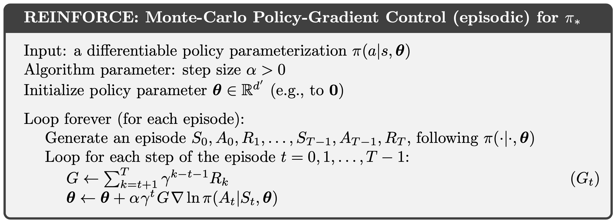
Where \(G_{t}\) is the return at \(t\), so for every \(t\), compute \(G_{t}\) for the update.
Actor Critic
Since the PG uses MC, it suffers from high variance. To remedy this, the actot critic (AC) is introduced, which employs a bootstrapping strategy in the PG. The AC parameterizes both the value function and policy, and 1) update the value functions with a bootstrapping to estimate the true value functions and 2) update the policy in respect to the estimated Q value to acquire higher value functions. The name is originated from the fact that the value function critizes (critic) the action selection from the policy (actor).
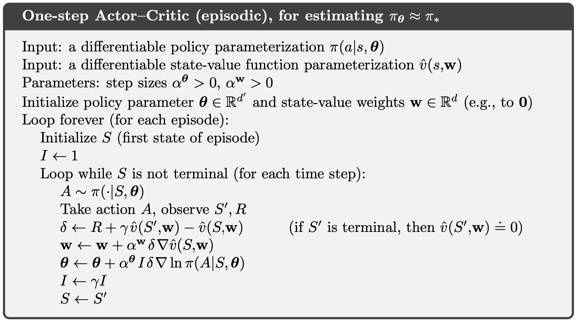
Where the temporal difference (TD) residual is used to compute \(\delta\). Unlike REINFORCE, one-step AC updates the parameters every time step.
Summary
The PG is an on-policy RL algorithm that finds the optimal policy using the MC method. Unlike value-based methods, the PG parameterizes the policy with a function approximator such that maximizes the return. The PG objective function has many equivalent expressions.
\[\begin{align} \mathcal{J} ( \theta ) & = \mathbb{E}_{ s \sim d^{\pi_{\theta}}, a \sim \pi_{\theta} } [ R ( s , a ) ] = \sum_{s \in \mathcal{S}} d^{\pi_{\theta}} ( s ) \sum_{a \in \mathcal{A}} \pi_{\theta} (a \vert s) R ( s , a ) \\ & \equiv \mathbb{E}_{ s \sim d^{\pi_{\theta}}, a \sim \pi_{\theta} } \left[ Q^{\pi_{\theta}} (s, a) \right] = \sum_{s \in \mathcal{S}} d^{\pi_{\theta}} ( s ) \sum_{a \in \mathcal{A}} \pi_{\theta} (a \vert s) Q^{\pi_{\theta}} (s, a) \\ & \equiv \mathbb{E}_{ s \sim d^{\pi_{\theta}} } \left[ V^{\pi_{\theta}} (s) \right] = \sum_{s \in \mathcal{S}} d^{\pi_{\theta}} ( s ) V^{\pi_{\theta}} (s) \\ & \equiv \mathbb{E}_{ s_{0} \sim p_{0} } \left[ V^{\pi_{\theta}} (s_{0}) \right] = \sum_{s_{0} \in \mathcal{S}} p_{0} ( s_{0} ) V^{\pi_{\theta}} (s_{0}) \end{align}\]- \[\begin{equation} \nabla_{\theta} \mathcal{J} ( \theta ) \propto \sum_{s \in \mathcal{S}} d^{\pi_{\theta}} ( s ) \sum_{a \in \mathcal{A}} \pi_{\theta} (a \vert s) Q^{\pi_{\theta}} (s, a) \nabla_{\theta} \pi_{\theta} (a \vert s) = \mathbb{E}_{ s \sim d^{\pi_{\theta}}, a \sim \pi_{\theta} } \left[ Q^{\pi_{\theta}} (s, a) \nabla_{\theta} \ln \pi_{\theta} (a \vert s) \right] \end{equation}\]
-
Theorem 2 (Policy Gradient with Function Approximation):
\[\begin{equation} \nabla_{ \theta } \mathcal{J} (\theta) \propto \mathbb{E}_{ s \sim d^{\pi_{\theta}} , a \sim \pi_{\theta} } \left[ Q^{\pi_{\theta}} (s, a) \nabla_{ \theta} \ln \pi_{\theta} (a \vert s) \right] \equiv \mathbb{E}_{ s \sim d^{\pi_{\theta}} , a \sim \pi_{\theta} } \left[ Q_{ \phi } (s, a) \nabla_{ \theta} \ln \pi_{\theta} (a \vert s) \right] \end{equation}\]- Where two conditions must meet.
- There are two types of policy distribution that meet the two conditions.
- Softmax policy distribution for discrete action space.
- Gaussian policy distribution for continuous action space.
The DPG is just the PG with the greedy policy, developed to improve computational efficiency in continuous state and action space.
\[\begin{align} \mathcal{J} ( \theta ) & = \mathbb{E}_{ s \sim d^{\mu_{\theta}} } [ R ( s , \mu_{\theta} ( s ) ) ] = \int_{\mathcal{S}} d^{\mu_{\theta}} ( s ) R ( s , \mu_{\theta} ( s ) ) \text{ d}s \\ & \equiv \mathbb{E}_{ s \sim d^{\mu_{\theta}} } \left[ Q^{\mu_{\theta}} (s, \mu_{\theta} ( s )) \right] = \int_{\mathcal{S}} d^{\mu_{\theta}} ( s ) Q^{\mu_{\theta}} (s, \mu_{\theta} ( s )) \text{ d}s \\ & \equiv \mathbb{E}_{ s \sim d^{\mu_{\theta}} } \left[ V^{\mu_{\theta}} (s) \right] = \int_{\mathcal{S}} d^{\mu_{\theta}} ( s ) V^{\mu_{\theta}} (s) \text{ d}s \\ & \equiv \mathbb{E}_{ s_{0} \sim p_{0} } \left[ V^{\mu_{\theta}} (s_{0}) \right] = \int_{\mathcal{S}} p_{0} ( s_{0} ) V^{\mu_{\theta}} (s_{0}) \text{ d}s_{0} \end{align}\]- \[\begin{align} \nabla_{\theta} \mathcal{J} ( \theta ) & = \nabla_{\theta} \int_{\mathcal{S}} d^{\mu_{\theta}} ( s ) Q^{\mu_{\theta}} (s, \mu_{\theta} ( s )) \text{ d}s = \mathbb{E}_{ s \sim d^{\mu_{\theta}} } \left[ \nabla_{\theta} Q^{\mu_{\theta}} (s, \mu_{\theta} ( s )) \right] \\ & \propto \int_{\mathcal{S}} d^{\mu_{\theta}} ( s ) \nabla_{ \theta} \mu_{\theta} ( s ) \nabla_{ a } Q^{\mu_{\theta}} (s, a) \vert_{a = \mu_{\theta} ( s )} \text{ d}s = \mathbb{E}_{ s \sim d^{\mu_{\theta}} } \left[ \nabla_{ \theta} \mu_{\theta} ( s ) \nabla_{ a } Q^{\mu_{\theta}} (s, a) \vert_{a = \mu_{\theta} ( s )} \right] \end{align}\]
- \[\begin{equation} \lim_{\sigma \rightarrow 0} \nabla_{\theta} \mathcal{J} ( \pi_{ \mu_{\theta}, \sigma } ) = \nabla_{\theta} \mathcal{J} ( \mu_{\theta} ) \end{equation}\]
-
Theorem 3 (Compatible Function Approximation):
\[\begin{equation} \nabla_{ \theta } \mathcal{J} (\theta) \propto \mathbb{E}_{ s \sim d^{\mu_{\theta}} } \left[ \nabla_{ a } Q^{\mu_{\theta}} (s, a) \vert_{a = \mu_{\theta} ( s )} \nabla_{ \theta} \mu_{\theta} ( s ) \right] \equiv \mathbb{E}_{ s \sim d^{\mu_{\theta}} } \left[ \nabla_{ a } Q_{\phi} (s, a) \vert_{a = \mu_{\theta} ( s )} \nabla_{ \theta} \mu_{\theta} ( s ) \right] \end{equation}\]- Where two conditions must meet.
Three popular model-based algorithms are:
- The QL:
- parameterizes the value function.
- naturally encapsulates the deterministic policy.
- handles the MDP with only the discrete state/action space.
- updates per step using a bootstrapping.
- has relatively low variance, so it converges fast.
- has relatively high bias, so it may be more likely to fall into local optima.
- has initialization bias, so the initialization influences the final performance.
- has overestimation bias, so it takes a risky path.
- is naturally off-policy, so it has better exploration.
- The PG:
- parameterizes the policy.
- naturally encapsulates the stochastic policy.
- handles the MDP with both the discrete and continuous state/action space.
- updates per episode.
- has relatively high variance, so it converges slow.
- has relatively low bias, so it may be less likely to fall into local optima.
- is naturally on-policy, but off-policy can be employed with the importance sampling.
- The AC:
- parameterizes the value function and the policy.
- naturally encapsulates the stochastic policy.
- handles the MDP with both the discrete and continuous state/action space.
- updates per step using a bootstrapping.
- has relatively low variance, so it converges fast.
- has relatively low bias, so it may be less likely to fall into local optima.
- is naturally on-policy, but off-policy can be employed with the importance sampling.
Reference
- Policy Gradient Methods for Reinforcement Learning with Function Approximation
- Deterministic Policy Gradient Algorithms
- Chapter 13 in Reinforcement Learning: An Introduction
Other helpful resources are:
Comments